单个预测的 SHAP 瀑布图
每项特征如何把一个困难学区的预测数学成绩从平均值推到模型的输出。
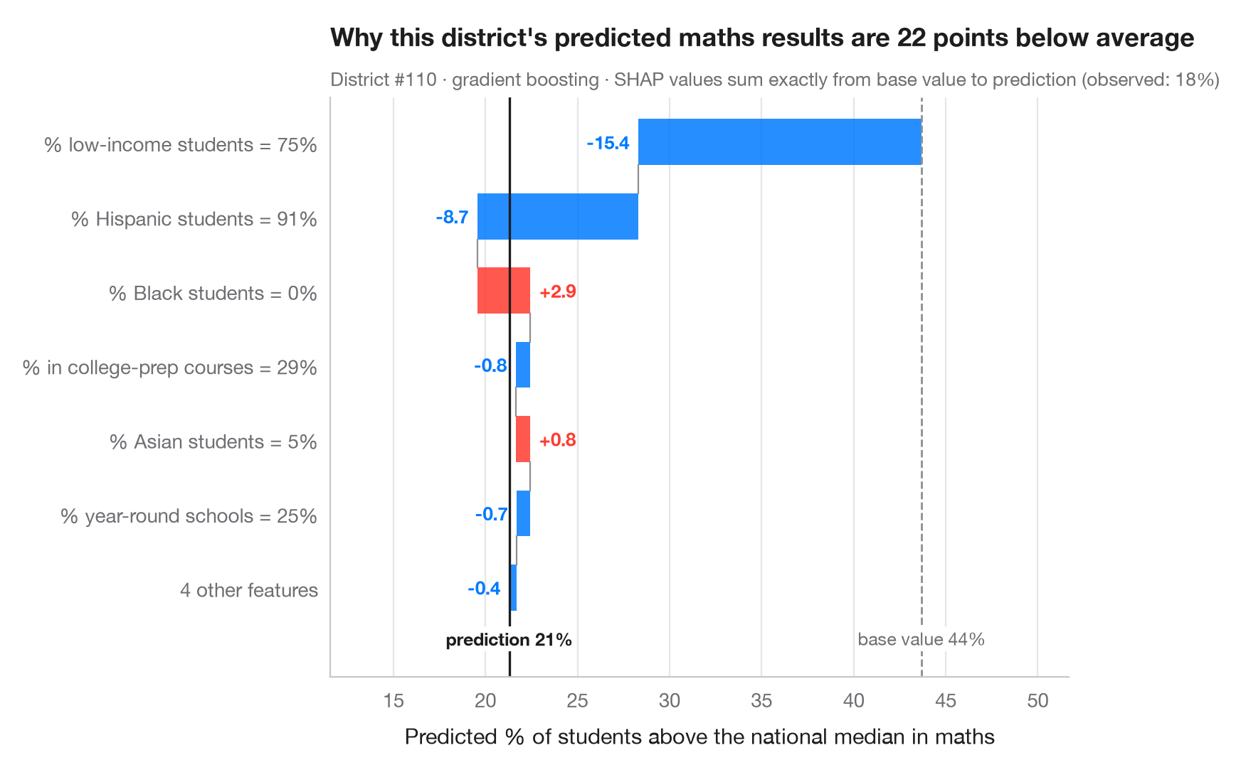
全局图形描述的是模型;瀑布图解释的是 一个 预测。它从基准值——模型在数据上的平均预测——出发,按从大到小的顺序依次加上每个特征的 SHAP 值,直到得到这个学区的预测值。红色条把预测推高,蓝色条把预测拉低;最小的若干贡献合并为一条,以保持图形清晰。由于 SHAP 值可加,各条之和总是恰好等于基准值与预测值之差。
当需要解释单个个案时——一个被列为扶持对象的学区、一笔贷款、一份福利申请——就该展示这张图。它解释的是 模型 做了什么,而不是结果为何发生。数据为 statsmodels 自带的 1998 年 STAR 考试中加利福尼亚州 303 个学区(sm.datasets.star98);结果变量为数学成绩高于全国中位数的学生占比,由学区的十项特征预测。模型为梯度提升回归;SHAP 值来自 shap.TreeExplainer。所示学区为困难个案(预测值低于基准值 20 个百分点以上),之所以选择它,是因为其解释同时包含正反两个方向的作用。
代码及图中文字均为英文。
import matplotlib.pyplot as plt
import numpy as np
import shap
import statsmodels.api as sm
from sklearn.ensemble import GradientBoostingRegressor

# Data: 303 California school districts; outcome = % of students above the national median in maths
d = sm.datasets.star98.load_pandas().data
y = 100 * d["NABOVE"] / (d["NABOVE"] + d["NBELOW"])
names = {"LOWINC": "% low-income students", "PERASIAN": "% Asian students", "PERBLACK": "% Black students",
         "PERHISP": "% Hispanic students", "AVYRSEXP": "Teacher experience (years)",
         "AVSALK": "Teacher salary ($000)", "PERSPENK": "Spending per pupil ($000)",
         "PTRATIO": "Pupils per teacher", "PCTAF": "% in college-prep courses",
         "PCTYRRND": "% year-round schools"}
X = d[list(names)]
fmt = {"LOWINC": "{:.0f}%", "PERASIAN": "{:.0f}%", "PERBLACK": "{:.0f}%", "PERHISP": "{:.0f}%",
       "AVYRSEXP": "{:.1f}", "AVSALK": "{:.1f}", "PERSPENK": "{:.2f}", "PTRATIO": "{:.1f}",
       "PCTAF": "{:.0f}%", "PCTYRRND": "{:.0f}%"}
model = GradientBoostingRegressor(learning_rate=0.05, n_estimators=300, max_depth=2,
                                  subsample=0.8, random_state=0).fit(X, y)

explainer = shap.TreeExplainer(model)
base = float(np.ravel(explainer.expected_value)[0])
all_sv = explainer.shap_values(X)
# A struggling district whose explanation has pushes in both directions
low = np.where(all_sv.sum(axis=1) < -20)[0]
p = int(low[np.argmax(all_sv[low].max(axis=1))])
sv = all_sv[p]

# Largest contributions first; pool the rest
k = 6
idx = np.argsort(np.abs(sv))[::-1]
top, rest = idx[:k], idx[k:]
labels = [f"{names[X.columns[j]]} = {fmt[X.columns[j]].format(X.iloc[p, j])}" for j in top]
values = list(sv[top])
if len(rest):
    labels.append(f"{len(rest)} other features")
    values.append(sv[rest].sum())

fig, ax = plt.subplots(figsize=(8, 5.2))
start = base
for i, (lab, v) in enumerate(zip(labels, values)):
    c = "#FF3B30" if v > 0 else "#007AFF"
    ax.barh(i, v, left=start, color=c, alpha=0.85, height=0.62)
    ax.text(start + v + (0.5 if v > 0 else -0.5), i, f"{v:+.1f}", va="center",
            ha="left" if v > 0 else "right", fontsize=9.5, color=c, fontweight="semibold")
    if i < len(values) - 1:
        ax.plot([start + v] * 2, [i + 0.31, i + 0.69], color="#8E8E93", lw=0.8)
    start += v
ax.axvline(base, color="#8E8E93", ls="--", lw=1)
ax.axvline(start, color="#1d1d1f", lw=1.2)
bottom = len(labels) - 0.45
ax.text(base, bottom, f"base value {base:.0f}%", ha="center", va="top", fontsize=9, color="#6E6E73",
        bbox=dict(fc="white", ec="none", pad=1))
ax.text(start, bottom, f"prediction {start:.0f}%", ha="center", va="top", fontsize=9,
        color="#1d1d1f", fontweight="semibold", bbox=dict(fc="white", ec="none", pad=1))
ax.set_yticks(range(len(labels)), labels)
ax.set_ylim(len(labels) + 0.2, -0.6)
lo_x = min(base, *(base + np.cumsum(values)))
ax.set_xlim(lo_x - 8, max(base, *(base + np.cumsum(values))) + 8)
ax.set_xlabel("Predicted % of students above the national median in maths")
ax.grid(axis="x"); ax.grid(axis="y", visible=False)
ax.set_title(f"Why this district's predicted maths results are {base - start:.0f} points below average", pad=26)
ax.text(0, 1.02, f"District #{p} · gradient boosting · SHAP values sum exactly from base value to prediction "
        f"(observed: {y.iloc[p]:.0f}%)", transform=ax.transAxes, fontsize=9.5, color="#6E6E73")
plt.show()
图表使用了可选的 PyStatlas 样式:添加 plt.style.use("pystatlas.mplstyle") 即可完全还原其外观。
数据来源
- California STAR test results, 1998 (303 school districts). Gill, J. (2001). Generalized Linear Models: A Unified Approach (Quantitative Applications in the Social Sciences, No. 134). Sage. https://www.statsmodels.org/stable/datasets/generated/star98.html
Original data from the California Department of Education's Standardized Testing and Reporting (STAR) program, 1998. Subset distributed with statsmodels (sm.datasets.star98) with the author's permission.
这些示例用于说明统计方法。图表标题描述的是该图在这些特定数据中呈现的内容——这些数据往往样本较小、年代较早或并不完整——而不是作者对实质问题的立场。关于解释、背景和数据质量,请以此处引用的原始来源为准。
如何引用
PyStatlas 由 Thierry Warin 创建并维护。如果它对你的工作有所帮助,敬请引用。
Warin, T. (2026). SHAP waterfall for one prediction. In PyStatlas: A Python Gallery of Statistical Graphics for the Social Sciences. https://warint.github.io/pystatlas/machine-learning/shap-waterfall/
@misc{warin2026statlas,
  author       = {Warin, Thierry},
  title        = {PyStatlas: A Python Gallery of Statistical Graphics for the Social Sciences},
  year         = {2026},
  howpublished = {\url{https://warint.github.io/pystatlas/}},
  note         = {Source code: https://github.com/warint/pystatlas}
}