SHAP dependence plot — PyStatlas: A Python Gallery of Statistical Graphics for the Social Sciences

Warin, Thierry

SHAP 依存プロット

低所得世帯の生徒の割合が各学区の予測される数学の成績にどう効くかを、最も強い交互作用の相手で色分けし、平滑化した傾向線を添えて示します。

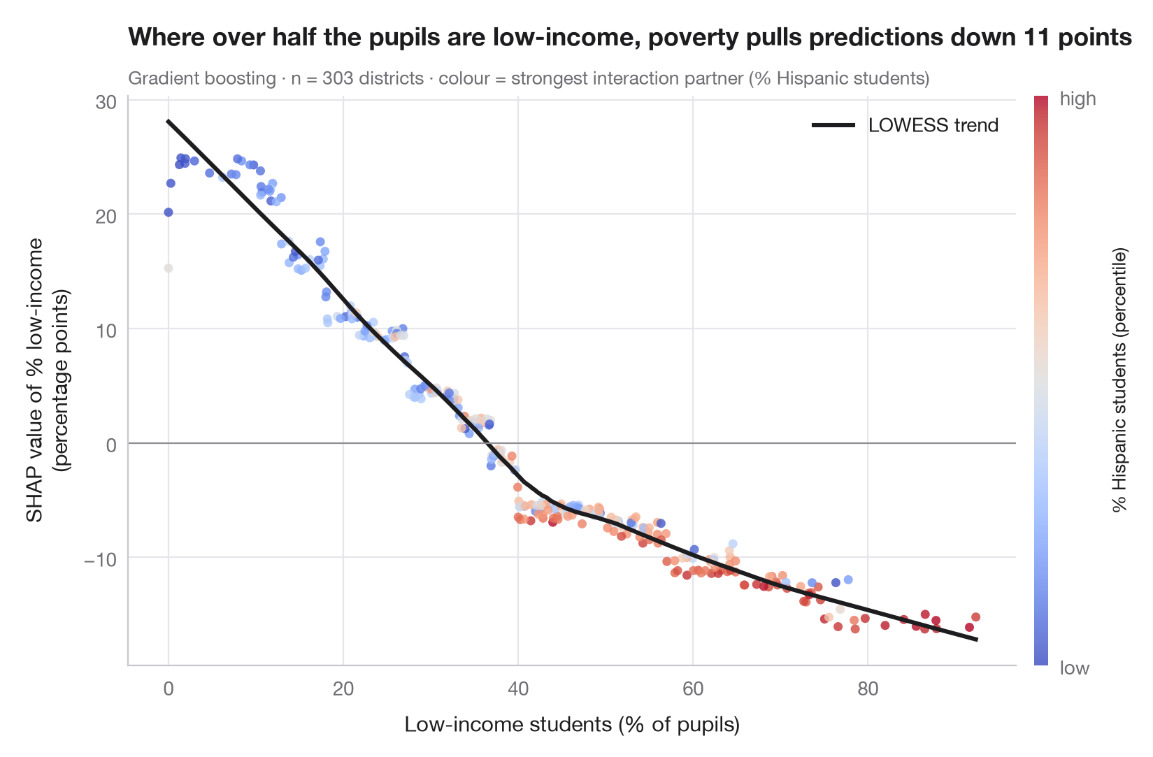
SHAP 依存プロットは 1 つの特徴量に焦点を当てます。各点が学区で、横軸は特徴量の値、縦軸はその SHAP 値、すなわちその学区の予測への寄与です。傾向線（LOWESS 平滑化）は部分依存曲線に近いものですが、その周りの点の広がりにも情報があります。低所得世帯の生徒の割合が同じでも、ほかの特徴量との 交互作用 によって寄与は学区ごとに異なるのです。

色は、この縦方向の広がりを最もよく説明する特徴量を示します。ここでは低所得世帯の生徒の割合との SHAP 交互作用 値が平均して最も大きい特徴量を選んでいます（shap.TreeExplainer.shap_interaction_values）。ここではそれはヒスパニック系の生徒の割合で、これ自体が貧困と強く相関している（r ≈ 0.7）ため、色のグラデーションの一部は交互作用ではなくこの相関を反映しています。データは statsmodels 付属の 1998 年 STAR テストにおけるカリフォルニア州の学区 303 件（sm.datasets.star98）で、目的変数は数学で全国中央値を上回った生徒の割合、これを学区の 10 の特性から予測します。モデルは勾配ブースティング回帰、平滑化は statsmodels.nonparametric.lowess によります。

コードおよび図中のテキストは英語です。

shap-dependence.py · 50 行

ダウンロード GitHub

import matplotlib.pyplot as plt
import numpy as np
import shap
import statsmodels.api as sm
from sklearn.ensemble import GradientBoostingRegressor
from statsmodels.nonparametric.smoothers_lowess import lowess

# Data: 303 California school districts; outcome = % of students above the national median in maths
d = sm.datasets.star98.load_pandas().data
y = 100 * d["NABOVE"] / (d["NABOVE"] + d["NBELOW"])
names = {"LOWINC": "% low-income students", "PERASIAN": "% Asian students", "PERBLACK": "% Black students",
         "PERHISP": "% Hispanic students", "AVYRSEXP": "Teacher experience (years)",
         "AVSALK": "Teacher salary ($000)", "PERSPENK": "Spending per pupil ($000)",
         "PTRATIO": "Pupils per teacher", "PCTAF": "% in college-prep courses",
         "PCTYRRND": "% year-round schools"}
X = d[list(names)]
model = GradientBoostingRegressor(learning_rate=0.05, n_estimators=300, max_depth=2,
                                  subsample=0.8, random_state=0).fit(X, y)

explainer = shap.TreeExplainer(model)
sv = explainer.shap_values(X)
inter = explainer.shap_interaction_values(X)            # (districts, features, features)

f = list(X.columns).index("LOWINC")
strength = np.abs(inter[:, f, :]).mean(axis=0)
strength[f] = 0
partner = int(np.argmax(strength))                       # strongest interaction partner

x, s = X.iloc[:, f].to_numpy(), sv[:, f]
col = X.iloc[:, partner].rank(pct=True).to_numpy()
trend = lowess(s, x, frac=0.35)

fig, ax = plt.subplots(figsize=(8, 5.2))
sc = ax.scatter(x, s, c=col, cmap="coolwarm", s=22, alpha=0.8, lw=0, vmin=0, vmax=1)
ax.plot(trend[:, 0], trend[:, 1], color="#1d1d1f", lw=2.2, label="LOWESS trend")
ax.axhline(0, color="#8E8E93", lw=0.8)
ax.set_xlabel("Low-income students (% of pupils)")
ax.set_ylabel("SHAP value of % low-income\n(percentage points)")
ax.grid(axis="x")
ax.legend(loc="upper right")
cb = fig.colorbar(sc, ax=ax, pad=0.02, aspect=40, ticks=[0, 1])
cb.ax.set_yticklabels(["low", "high"])
cb.set_label(f"{names[X.columns[partner]]} (percentile)", fontsize=9.5)
cb.outline.set_visible(False)

above = s[x > 50].mean()
ax.set_title(f"Where over half the pupils are low-income, poverty pulls predictions down {-above:.0f} points", pad=26)
ax.text(0, 1.02, f"Gradient boosting · n = {len(X)} districts · colour = strongest interaction "
        f"partner ({names[X.columns[partner]]})", transform=ax.transAxes, fontsize=9.5, color="#6E6E73")
plt.show()

図にはオプションの PyStatlas スタイルを使用しています。同じ見た目にするには plt.style.use("pystatlas.mplstyle") を追加してください。

データの出典

California STAR test results, 1998 (303 school districts). Gill, J. (2001). Generalized Linear Models: A Unified Approach (Quantitative Applications in the Social Sciences, No. 134). Sage. https://www.statsmodels.org/stable/datasets/generated/star98.html
Original data from the California Department of Education's Standardized Testing and Reporting (STAR) program, 1998. Subset distributed with statsmodels (sm.datasets.star98) with the author's permission.

これらの例は統計手法を説明するためのものです。図のタイトルは、この特定のデータ（多くは小規模で、古く、部分的な標本）で図が示す内容を述べたものであり、実質的な問いに対する著者の立場ではありません。解釈、背景、データの質については、ここに挙げた元の出典を参照してください。

引用方法

PyStatlas は Thierry Warin が作成・運営しています。研究や業務に役立った場合は、ぜひ引用してください。

Warin, T. (2026). SHAP dependence plot. In PyStatlas: A Python Gallery of Statistical Graphics for the Social Sciences. https://warint.github.io/pystatlas/machine-learning/shap-dependence/

@misc{warin2026statlas,
  author       = {Warin, Thierry},
  title        = {PyStatlas: A Python Gallery of Statistical Graphics for the Social Sciences},
  year         = {2026},
  howpublished = {\url{https://warint.github.io/pystatlas/}},
  note         = {Source code: https://github.com/warint/pystatlas}
}

機械学習のその他のグラフ

機械学習

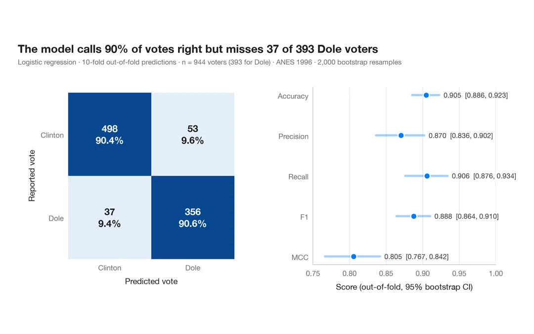
指標付き混同行列

1996 年にドールに投票した人をロジスティック回帰がどれだけ当てられるか。件数と行ごとの割合を示す交差検証の混同行列に、主要指標のブートストラップ区間を添えます。

yardstick::conf_mat() + autoplot()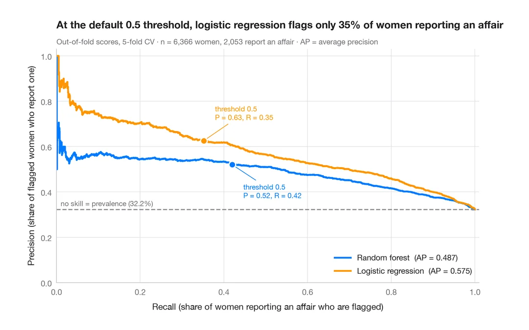

機械学習

適合率–再現率曲線

既婚女性のうち誰が婚外関係を申告するかを予測する 2 つの分類器の、交差検証による適合率–再現率曲線と、平均適合率、無技能のベースライン。

yardstick::pr_curve() + autoplot()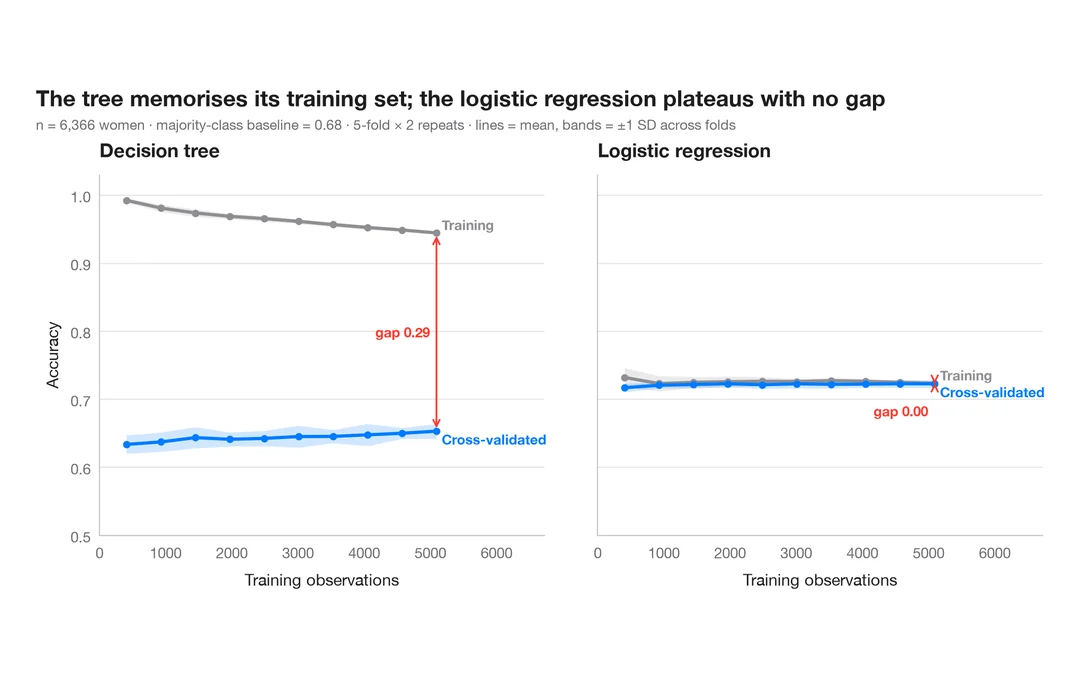

機械学習

学習曲線

既婚女性のうち誰が婚外関係を申告するかを予測する 2 つのモデルについて、訓練データを増やしたときの訓練正解率と交差検証正解率を示します。

caret::learning_curve_dat() + ggplot()