预测概率
按组绘制随某一预测变量变化的模型预测概率曲线,附 95% 置信带。
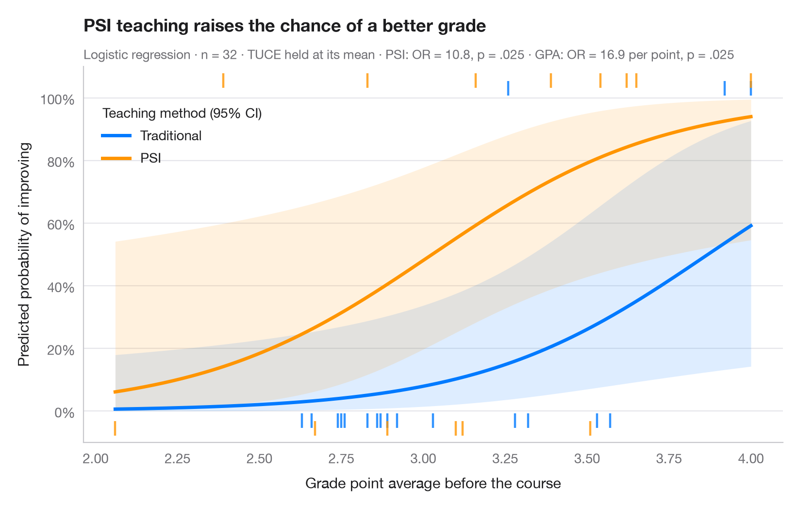
优势比难以直观感受,概率则不然。这张图将 logistic 模型还原到结局尺度:每条曲线是某个因素水平下,成功的预测概率随一个连续预测变量取值范围的变化,其他协变量固定在均值。置信带是在 logit 尺度上计算后再反变换的 95% 置信区间,因此始终位于 [0, 1] 之内。地毯线标示观测到的学生——成绩提高者位于顶部,未提高者位于底部。
数据为 statsmodels 自带的 Spector & Mazzeo(1980)实验(sm.datasets.spector):在控制此前 GPA 和前测成绩(TUCE)后,一种新的教学方法(PSI)能否提高成绩?模型为二项 smf.glm();曲线来自 get_prediction().summary_frame()。
代码及图中文字均为英文。
import matplotlib.pyplot as plt
import numpy as np
import pandas as pd
import statsmodels.api as sm
import statsmodels.formula.api as smf

# Data: 32 students; GRADE = 1 if the grade improved after the course
df = sm.datasets.spector.load_pandas().data
model = smf.glm("GRADE ~ GPA + TUCE + C(PSI)", data=df, family=sm.families.Binomial()).fit()

# Prediction grid: GPA across its range, TUCE at its mean, both teaching methods
gpa = np.linspace(df.GPA.min(), df.GPA.max(), 200)
groups = {0: ("Traditional", "#007AFF"), 1: ("PSI", "#FF9500")}

fig, ax = plt.subplots(figsize=(8, 5))
for level, (name, c) in groups.items():
    grid = pd.DataFrame({"GPA": gpa, "TUCE": df.TUCE.mean(), "PSI": level})
    pred = model.get_prediction(grid).summary_frame(alpha=0.05)
    ax.fill_between(gpa, pred.mean_ci_lower, pred.mean_ci_upper, color=c, alpha=0.13, lw=0)
    ax.plot(gpa, pred["mean"], color=c, lw=2.5, label=name)
    # Rug of observations: improved (top) or not (bottom), slightly offset per group
    obs = df[df.PSI == level]
    y_rug = np.where(obs.GRADE == 1, 1.03 + 0.025 * level, -0.03 - 0.025 * level)
    ax.scatter(obs.GPA, y_rug, marker="|", s=110, lw=1.6, color=c, alpha=0.8, clip_on=False)

ax.legend(loc="upper left", title="Teaching method (95% CI)", alignment="left",
          bbox_to_anchor=(0.01, 0.93))
ax.set_ylim(-0.1, 1.1)
ax.set_yticks(np.linspace(0, 1, 6), [f"{v:.0%}" for v in np.linspace(0, 1, 6)])
ax.set_xlabel("Grade point average before the course")
ax.set_ylabel("Predicted probability of improving")
ax.set_title("PSI teaching raises the chance of a better grade", pad=26)
psi = "C(PSI)[T.1.0]"
fmt_p = lambda p: f"{p:.3f}".lstrip("0")
ax.text(0, 1.02, f"Logistic regression · n = {int(model.nobs)} · TUCE held at its mean · "
        f"PSI: OR = {np.exp(model.params[psi]):.1f}, p = {fmt_p(model.pvalues[psi])} · "
        f"GPA: OR = {np.exp(model.params['GPA']):.1f} per point, p = {fmt_p(model.pvalues['GPA'])}",
        transform=ax.transAxes, fontsize=9.5, color="#6E6E73")
plt.show()
图表使用了可选的 PyStatlas 样式:添加 plt.style.use("pystatlas.mplstyle") 即可完全还原其外观。
数据来源
- Spector and Mazzeo's teaching-method experiment (32 students). Spector, L. C., & Mazzeo, M. (1980). Probit analysis and economic education. Journal of Economic Education, 11(2), 37–44. https://www.statsmodels.org/stable/datasets/generated/spector.html
Obtained from W. Greene's Econometric Analysis web site with the original author's permission; distributed with statsmodels (sm.datasets.spector).
这些示例用于说明统计方法。图表标题描述的是该图在这些特定数据中呈现的内容——这些数据往往样本较小、年代较早或并不完整——而不是作者对实质问题的立场。关于解释、背景和数据质量,请以此处引用的原始来源为准。
如何引用
PyStatlas 由 Thierry Warin 创建并维护。如果它对你的工作有所帮助,敬请引用。
Warin, T. (2026). Predicted probabilities. In PyStatlas: A Python Gallery of Statistical Graphics for the Social Sciences. https://warint.github.io/pystatlas/regression-models/predicted-probabilities/
@misc{warin2026statlas,
  author       = {Warin, Thierry},
  title        = {PyStatlas: A Python Gallery of Statistical Graphics for the Social Sciences},
  year         = {2026},
  howpublished = {\url{https://warint.github.io/pystatlas/}},
  note         = {Source code: https://github.com/warint/pystatlas}
}