Partial dependence with ICE curves — PyStatlas: A Python Gallery of Statistical Graphics for the Social Sciences

Warin, Thierry

ICE 曲線付き部分依存プロット

予測される数学の成績が貧困と生徒 1 人あたり支出によってどう変わるか。平均（PDP）を学区ごとの曲線（ICE）に重ねて示します。

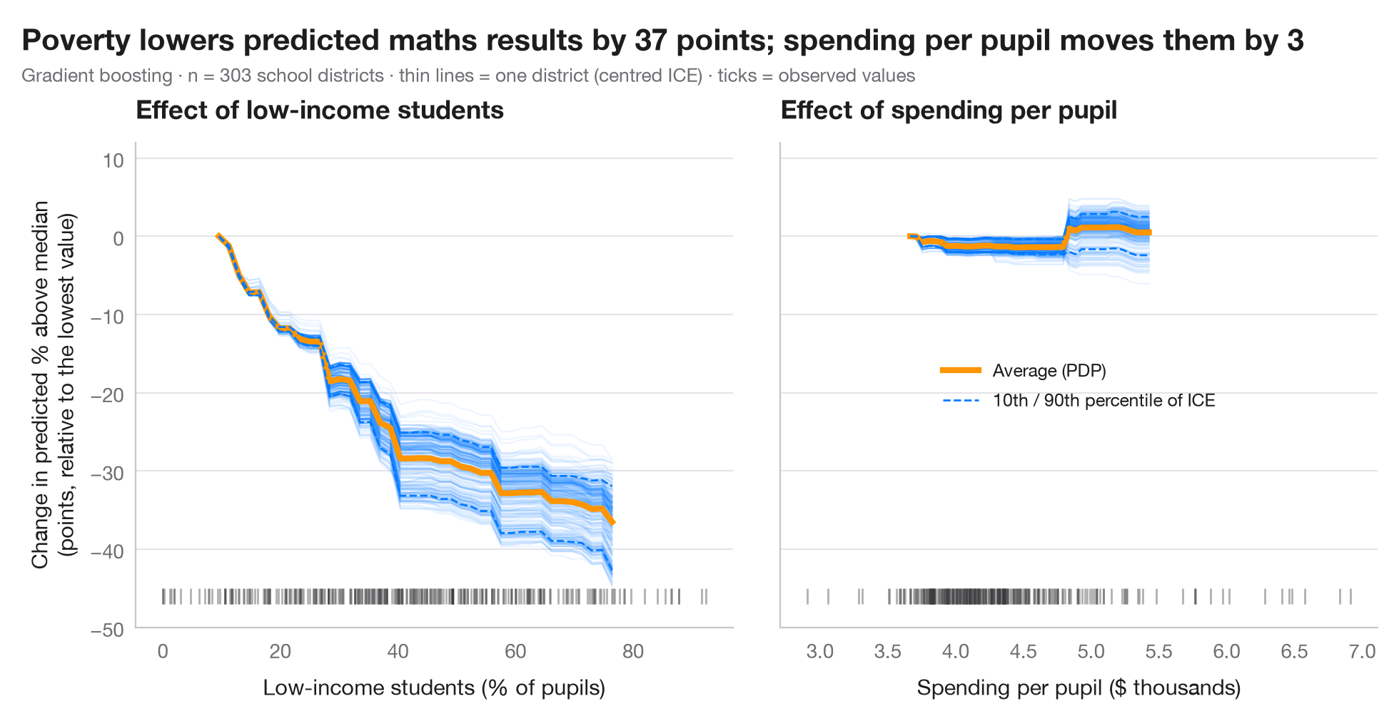
部分依存プロット（PDP）は、ほかの特徴量を観測値のまま保ち、1 つの特徴量を動かしたときに、モデルの予測が平均してどう変わるかを示します。その平均の背後には、観測値ごとに 1 本ずつの 個別条件付き期待値（ICE）曲線があります。ICE 曲線が平行なら効果は全員に共通、広がったり交差したりすれば、平均が隠している 交互作用 が現れています。ICE 曲線は左端で揃えて（中心化して）あり、水準ではなく形を比べられます。下の目盛りは実際にデータがある場所を示します。それ以外ではモデルは外挿しています。

データは statsmodels 付属の 1998 年 STAR テストにおけるカリフォルニア州の学区 303 件（sm.datasets.star98）で、目的変数は数学で全国中央値を上回った生徒の割合、これを学区の 10 の特性から予測します。2 つのパネルは、予測が急に下がる低所得世帯の生徒の割合と、予測がほとんど動かない生徒 1 人あたり支出とを対比しています。モデルは勾配ブースティング回帰で、曲線は sklearn.inspection.partial_dependence(kind="both") によります。PDP が描くのはモデルであって世界ではありません。モデルが因果的である場合にのみ、因果的な解釈ができます。

コードおよび図中のテキストは英語です。

partial-dependence.py · 46 行

ダウンロード GitHub

import matplotlib.pyplot as plt
import numpy as np
import statsmodels.api as sm
from sklearn.ensemble import GradientBoostingRegressor
from sklearn.inspection import partial_dependence

# Data: 303 California school districts; outcome = % of students above the national median in maths
d = sm.datasets.star98.load_pandas().data
y = 100 * d["NABOVE"] / (d["NABOVE"] + d["NBELOW"])
names = {"LOWINC": "% low-income students", "PERASIAN": "% Asian students", "PERBLACK": "% Black students",
         "PERHISP": "% Hispanic students", "AVYRSEXP": "Teacher experience (years)",
         "AVSALK": "Teacher salary ($000)", "PERSPENK": "Spending per pupil ($000)",
         "PTRATIO": "Pupils per teacher", "PCTAF": "% in college-prep courses",
         "PCTYRRND": "% year-round schools"}
X = d[list(names)]
model = GradientBoostingRegressor(learning_rate=0.05, n_estimators=300, max_depth=2,
                                  subsample=0.8, random_state=0).fit(X, y)

features = {"LOWINC": "Low-income students (% of pupils)", "PERSPENK": "Spending per pupil ($ thousands)"}
change = {}
plt.rcParams["figure.constrained_layout.use"] = False   # manual margins leave room for the subtitle
fig, axes = plt.subplots(1, 2, figsize=(10, 5), sharey=True)
fig.subplots_adjust(left=0.10, right=0.97, top=0.80, bottom=0.12, wspace=0.08)
for ax, (f, label) in zip(axes, features.items()):
    pd_res = partial_dependence(model, X, [f], kind="both", grid_resolution=40)
    grid = pd_res["grid_values"][0]
    ice = pd_res["individual"][0]
    ice_c = ice - ice[:, [0]]                      # centred ICE
    pdp_c = pd_res["average"][0] - pd_res["average"][0][0]
    change[f] = np.ptp(pdp_c)                      # range of the average effect
    ax.plot(grid, ice_c.T, color="#007AFF", alpha=0.07, lw=0.8)
    ax.plot(grid, pdp_c, color="#FF9500", lw=3, label="Average (PDP)")
    lo, hi = np.percentile(ice_c, [10, 90], axis=0)
    ax.plot(grid, lo, color="#007AFF", lw=1, ls="--")
    ax.plot(grid, hi, color="#007AFF", lw=1, ls="--", label="10th / 90th percentile of ICE")
    ax.plot(X[f], np.full(len(X), -46), "|", color="#3A3A3C", ms=8, alpha=0.4)   # rug
    ax.set_xlabel(label)
    ax.set_title(f"Effect of {label.split(' (')[0].lower()}")
axes[0].set_ylim(-50, 12)
axes[0].set_ylabel("Change in predicted % above median\n(points, relative to the lowest value)")
axes[1].legend(loc="center", fontsize=9)
fig.suptitle(f"Poverty lowers predicted maths results by {change['LOWINC']:.0f} points; "
             f"spending per pupil moves them by {change['PERSPENK']:.0f}", x=0.02, y=0.97, ha="left")
fig.text(0.02, 0.885, f"Gradient boosting · n = {len(X)} school districts · thin lines = one district (centred ICE) · "
         "ticks = observed values", fontsize=9.5, color="#6E6E73")
plt.show()

図にはオプションの PyStatlas スタイルを使用しています。同じ見た目にするには plt.style.use("pystatlas.mplstyle") を追加してください。

データの出典

California STAR test results, 1998 (303 school districts). Gill, J. (2001). Generalized Linear Models: A Unified Approach (Quantitative Applications in the Social Sciences, No. 134). Sage. https://www.statsmodels.org/stable/datasets/generated/star98.html
Original data from the California Department of Education's Standardized Testing and Reporting (STAR) program, 1998. Subset distributed with statsmodels (sm.datasets.star98) with the author's permission.

これらの例は統計手法を説明するためのものです。図のタイトルは、この特定のデータ（多くは小規模で、古く、部分的な標本）で図が示す内容を述べたものであり、実質的な問いに対する著者の立場ではありません。解釈、背景、データの質については、ここに挙げた元の出典を参照してください。

引用方法

PyStatlas は Thierry Warin が作成・運営しています。研究や業務に役立った場合は、ぜひ引用してください。

Warin, T. (2026). Partial dependence with ICE curves. In PyStatlas: A Python Gallery of Statistical Graphics for the Social Sciences. https://warint.github.io/pystatlas/machine-learning/partial-dependence/

@misc{warin2026statlas,
  author       = {Warin, Thierry},
  title        = {PyStatlas: A Python Gallery of Statistical Graphics for the Social Sciences},
  year         = {2026},
  howpublished = {\url{https://warint.github.io/pystatlas/}},
  note         = {Source code: https://github.com/warint/pystatlas}
}

機械学習のその他のグラフ

機械学習

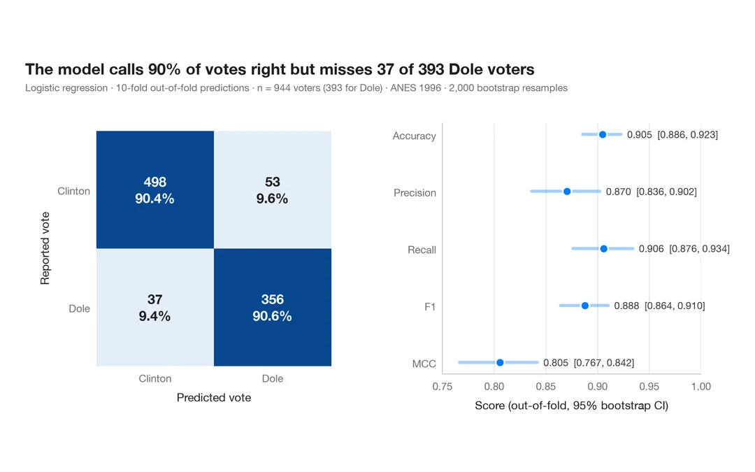
指標付き混同行列

1996 年にドールに投票した人をロジスティック回帰がどれだけ当てられるか。件数と行ごとの割合を示す交差検証の混同行列に、主要指標のブートストラップ区間を添えます。

yardstick::conf_mat() + autoplot()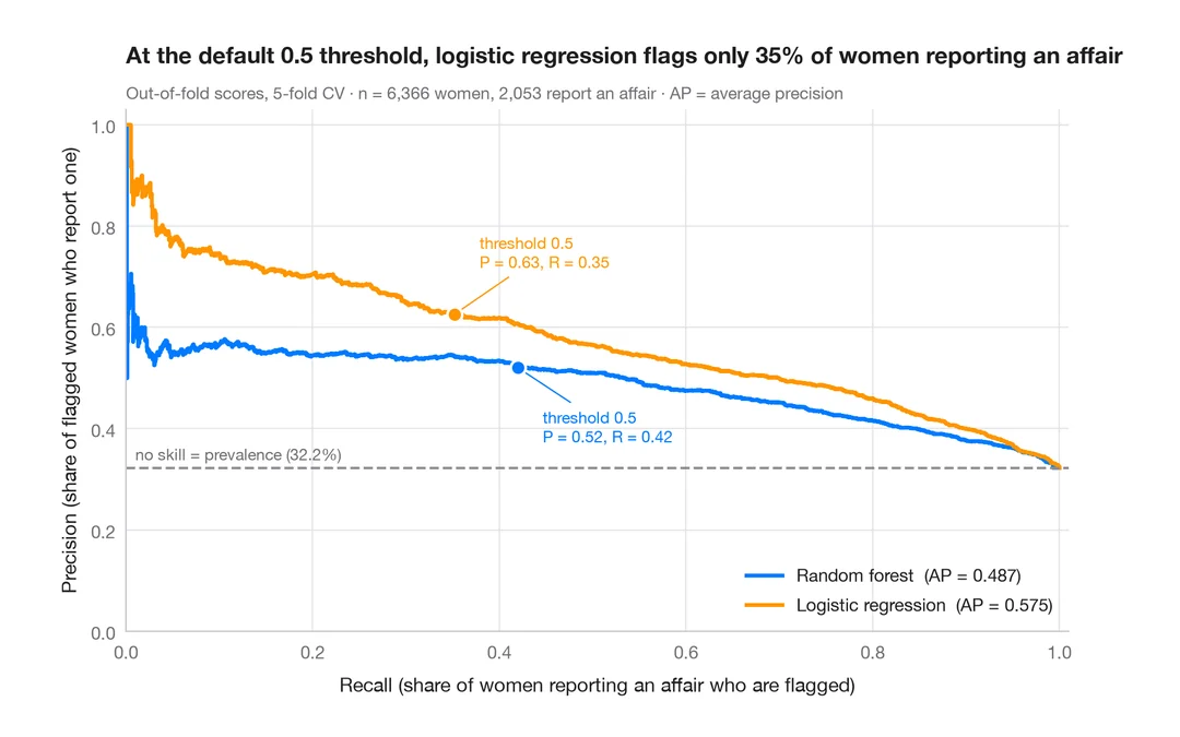

機械学習

適合率–再現率曲線

既婚女性のうち誰が婚外関係を申告するかを予測する 2 つの分類器の、交差検証による適合率–再現率曲線と、平均適合率、無技能のベースライン。

yardstick::pr_curve() + autoplot()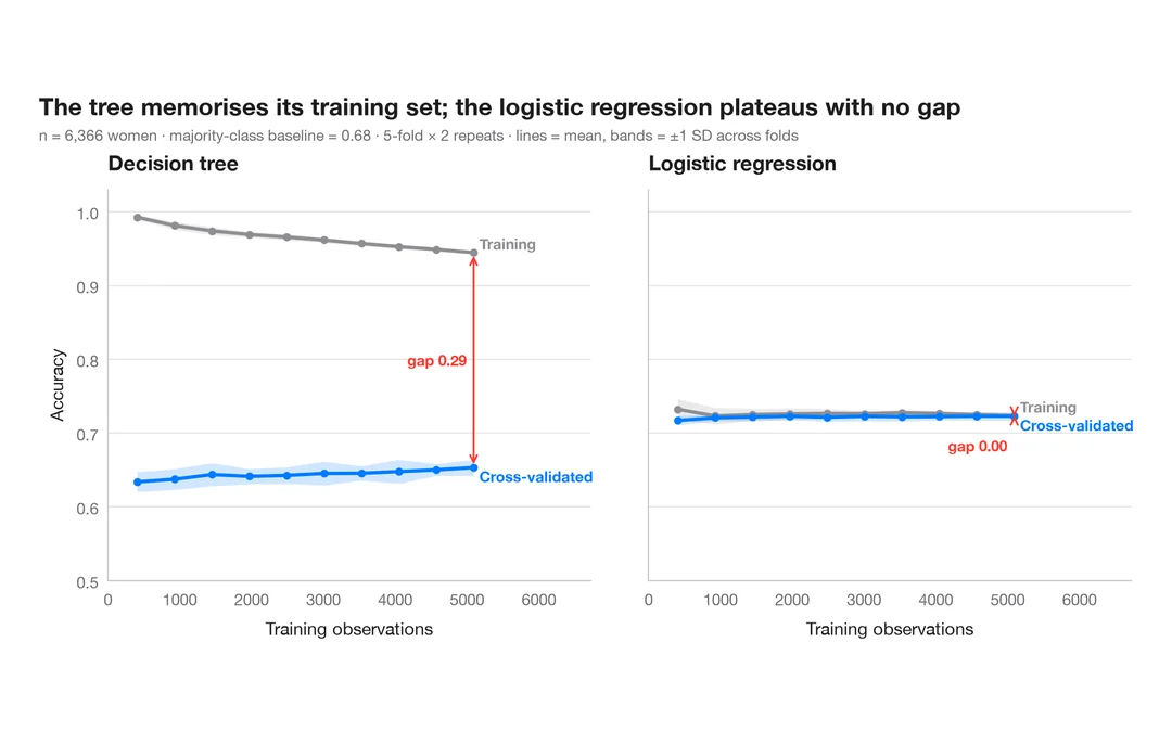

機械学習

学習曲線

既婚女性のうち誰が婚外関係を申告するかを予測する 2 つのモデルについて、訓練データを増やしたときの訓練正解率と交差検証正解率を示します。

caret::learning_curve_dat() + ggplot()