信頼区間付きの割合
群ごとの割合をウィルソンの 95% 信頼区間とともに、並べ替えたドットプロットで示します。
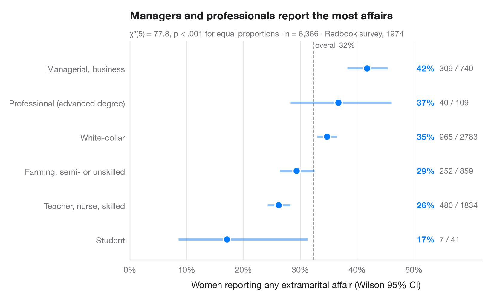
「各群のうちどれだけの割合が…?」という問いには、棒グラフよりも、群ごとの点と信頼区間のほうが適しています。目は位置を比較でき、区間の幅からどの群が小さいかがすぐにわかります。教科書的なワルド区間ではなく ウィルソンのスコア区間 を用いているのは、小さな群や 0 または 1 に近い割合でも 95% の被覆率を保てるためです。破線は全体の割合です。
データは statsmodels に同梱されている 1974年の Redbook 誌による既婚女性の調査(sm.datasets.fair)で、回答者の職業別に、婚外関係があったと回答した人の割合を示しています。区間は statsmodels.stats.proportion.proportion_confint(method="wilson") で求め、サブタイトルではすべての割合が等しいかどうかを scipy.stats.chi2_contingency で検定しています。
コードおよび図中のテキストは英語です。
import matplotlib.pyplot as plt
import numpy as np
import pandas as pd
import statsmodels.api as sm
from scipy import stats
from statsmodels.stats.proportion import proportion_confint

# Data: share of women reporting any affair, by occupation
df = sm.datasets.fair.load_pandas().data
jobs = {1: "Student", 2: "Farming, semi- or unskilled", 3: "White-collar",
        4: "Teacher, nurse, skilled", 5: "Managerial, business", 6: "Professional (advanced degree)"}
df["job"] = df.occupation.map(jobs)
df["affair"] = df.affairs > 0

# Proportion + Wilson 95% CI per group, sorted
g = df.groupby("job").affair.agg(k="sum", n="size")
g["p"] = g.k / g.n
g["low"], g["high"] = proportion_confint(g.k, g.n, alpha=0.05, method="wilson")
g = g.sort_values("p")

# Chi-squared test of homogeneity across the six groups
chi2, pval, dof, _ = stats.chi2_contingency(pd.crosstab(df.job, df.affair), correction=False)
overall = df.affair.mean()

fig, ax = plt.subplots(figsize=(8, 4.8))
y = np.arange(len(g))
ax.axvline(overall, color="#8E8E93", lw=1, ls="--", zorder=1)
ax.text(overall, len(g) - 0.45, f" overall {overall:.0%}", fontsize=9, color="#6E6E73", va="bottom")
ax.hlines(y, g.low, g.high, color="#007AFF", lw=2.5, alpha=0.45, zorder=2)
ax.scatter(g.p, y, s=80, color="#007AFF", edgecolor="white", lw=1.5, zorder=3)

for yi, (_, row) in zip(y, g.iterrows()):
    ax.text(0.505, yi, f"{row.p:.0%}", va="center", fontsize=10, fontweight="semibold", color="#007AFF")
    ax.text(0.545, yi, f"{row.k:.0f} / {row.n:.0f}", va="center", fontsize=9.5, color="#6E6E73")

ax.set_yticks(y, g.index)
ax.set_ylim(-0.6, len(g) - 0.2)
ax.set_xlim(0, 0.62)
ax.set_xticks(np.arange(0, 0.51, 0.1))
ax.xaxis.set_major_formatter(plt.matplotlib.ticker.PercentFormatter(1, decimals=0))
ax.grid(axis="x"); ax.grid(axis="y", visible=False)
ax.set_xlabel("Women reporting any extramarital affair (Wilson 95% CI)")
ax.set_title("Managers and professionals report the most affairs", pad=26)
ax.text(0, 1.02, f"χ²({dof}) = {chi2:.1f}, p < .001 for equal proportions · n = {len(df):,} · "
        "Redbook survey, 1974", transform=ax.transAxes, fontsize=9.5, color="#6E6E73")
plt.show()
図にはオプションの PyStatlas スタイル を使用しています。同じ見た目にするには plt.style.use("pystatlas.mplstyle") を追加してください。
データの出典
- Redbook survey of married women, 1974 (Fair's affairs data). Fair, R. C. (1978). A theory of extramarital affairs. Journal of Political Economy, 86(1), 45–61. https://doi.org/10.1086/260646
Data from the 1974 Redbook magazine survey; distributed with statsmodels (sm.datasets.fair) with the author's permission.
これらの例は統計手法を説明するためのものです。図のタイトルは、この特定のデータ(多くは小規模で、古く、部分的な標本)で図が示す内容を述べたものであり、実質的な問いに対する著者の立場ではありません。解釈、背景、データの質については、ここに挙げた元の出典を参照してください。
引用方法
PyStatlas は Thierry Warin が作成・運営しています。研究や業務に役立った場合は、ぜひ引用してください。
Warin, T. (2026). Proportions with confidence intervals. In PyStatlas: A Python Gallery of Statistical Graphics for the Social Sciences. https://warint.github.io/pystatlas/proportions-surveys/proportions-with-ci/
@misc{warin2026statlas,
  author       = {Warin, Thierry},
  title        = {PyStatlas: A Python Gallery of Statistical Graphics for the Social Sciences},
  year         = {2026},
  howpublished = {\url{https://warint.github.io/pystatlas/}},
  note         = {Source code: https://github.com/warint/pystatlas}
}