ピアソン残差付きモザイクプロット
セル度数に比例した面積のタイルを、独立性からのピアソン残差で色分けします。
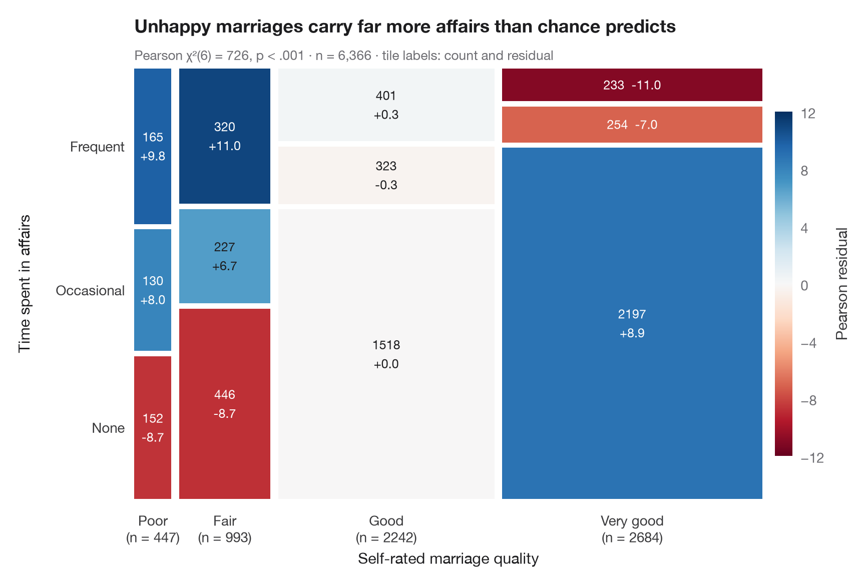
モザイクプロットは、二元表を正方形をタイルに分割した形で描きます。列の 幅 は第1変数の周辺割合、タイルの 高さ は第2変数の条件付き割合を表すため、各タイルの面積は度数に比例します。vcd::mosaic(shade = TRUE) と同様に、色は ピアソン残差 (observed − expected) / √expected を表します。青いタイルは独立性から予測されるより人数が多く、赤いタイルは少ないことを示し、±2 や ±4 を超える残差は χ² を押し上げているセルを示します。
データは statsmodels に同梱されている 1974年の Redbook 誌による既婚女性 6,366 人の調査(sm.datasets.fair)で、自己評価による結婚生活の満足度と婚外関係に費やした時間を対比しています。タイルは ax.bar で手作業で描き、期待度数は scipy.stats.chi2_contingency で求めています。
コードおよび図中のテキストは英語です。
import matplotlib.pyplot as plt
import numpy as np
import pandas as pd
import statsmodels.api as sm
from matplotlib.colors import TwoSlopeNorm
from scipy import stats

# Data: marriage rating (1-5, 1-2 pooled) × time spent in affairs (none / ≤ 1 / > 1)
df = sm.datasets.fair.load_pandas().data
rating = pd.cut(df.rate_marriage, [0, 2, 3, 4, 5], labels=["Poor", "Fair", "Good", "Very good"])
affairs = pd.cut(df.affairs, [-1, 0, 1, np.inf], labels=["None", "Occasional", "Frequent"])
table = pd.crosstab(rating, affairs)
obs = table.to_numpy()

# Chi-squared test and Pearson residuals
chi2, p, dof, expected = stats.chi2_contingency(obs, correction=False)
resid = (obs - expected) / np.sqrt(expected)

fig, ax = plt.subplots(figsize=(8.5, 5.6))
cmap = plt.get_cmap("RdBu")                         # red = fewer than expected, blue = more
norm = TwoSlopeNorm(0, vmin=-12, vmax=12)
gap = 0.012
widths = obs.sum(axis=1) / obs.sum()
x0 = 0
for i, w in enumerate(widths):
    heights = obs[i] / obs[i].sum()
    y0 = 0
    for j, h in enumerate(heights):
        ax.bar(x0, h - gap, width=w - gap, bottom=y0, align="edge",
               color=cmap(norm(resid[i, j])), edgecolor="none")
        sep = "  " if h < 0.12 else "\n"              # thin tiles get a one-line label
        ax.text(x0 + (w - gap) / 2, y0 + (h - gap) / 2, f"{obs[i, j]}{sep}{resid[i, j].round(1) + 0:+.1f}", ha="center", va="center",
                fontsize=9, linespacing=1.3, color="white" if abs(resid[i, j]) > 7 else "#1D1D1F")
        y0 += h
    ax.text(x0 + (w - gap) / 2, -0.03, f"{table.index[i]}\n(n = {obs[i].sum()})", ha="center", va="top",
            fontsize=10, color="#3A3A3C")
    x0 += w

# Row labels on the left, placed at the heights of the first column
y0 = 0
for j, h in enumerate(obs[0] / obs[0].sum()):
    ax.text(-0.015, y0 + (h - gap) / 2, table.columns[j], ha="right", va="center", fontsize=10, color="#3A3A3C")
    y0 += h

sm_ = plt.cm.ScalarMappable(norm=norm, cmap=cmap)
cb = fig.colorbar(sm_, ax=ax, shrink=0.8, pad=0.02, ticks=[-12, -8, -4, 0, 4, 8, 12])
cb.set_label("Pearson residual", color="#3A3A3C")
cb.outline.set_visible(False)
ax.set_xlim(0, 1 - gap); ax.set_ylim(0, 1 - gap)
ax.axis("off")
ax.text(0.5, -0.15, "Self-rated marriage quality", transform=ax.transAxes, ha="center", fontsize=11)
ax.text(-0.19, 0.5, "Time spent in affairs", transform=ax.transAxes, rotation=90, va="center", fontsize=11)
ax.set_title("Unhappy marriages carry far more affairs than chance predicts", pad=26)
ax.text(0, 1.02, f"Pearson χ²({dof}) = {chi2:.0f}, p < .001 · n = {obs.sum():,} · "
        "tile labels: count and residual", transform=ax.transAxes, fontsize=9.5, color="#6E6E73")
plt.show()
図にはオプションの PyStatlas スタイル を使用しています。同じ見た目にするには plt.style.use("pystatlas.mplstyle") を追加してください。
データの出典
- Redbook survey of married women, 1974 (Fair's affairs data). Fair, R. C. (1978). A theory of extramarital affairs. Journal of Political Economy, 86(1), 45–61. https://doi.org/10.1086/260646
Data from the 1974 Redbook magazine survey; distributed with statsmodels (sm.datasets.fair) with the author's permission.
これらの例は統計手法を説明するためのものです。図のタイトルは、この特定のデータ(多くは小規模で、古く、部分的な標本)で図が示す内容を述べたものであり、実質的な問いに対する著者の立場ではありません。解釈、背景、データの質については、ここに挙げた元の出典を参照してください。
引用方法
PyStatlas は Thierry Warin が作成・運営しています。研究や業務に役立った場合は、ぜひ引用してください。
Warin, T. (2026). Mosaic plot with Pearson residuals. In PyStatlas: A Python Gallery of Statistical Graphics for the Social Sciences. https://warint.github.io/pystatlas/proportions-surveys/mosaic-plot/
@misc{warin2026statlas,
  author       = {Warin, Thierry},
  title        = {PyStatlas: A Python Gallery of Statistical Graphics for the Social Sciences},
  year         = {2026},
  howpublished = {\url{https://warint.github.io/pystatlas/}},
  note         = {Source code: https://github.com/warint/pystatlas}
}