Some of the most important quantities in international business are not measured, because they cannot be. Absorptive capacity, institutional quality, brand strength, digital maturity — each is meant to be a real property of a firm or a country, each is invoked in explanations, and none of them appears in any dataset. What appears instead is a set of indicators, each a noisy and partial reflection of the thing.
Chapter 7 met this and handled it descriptively: factor analysis found a small number of common factors behind a battery of correlated items. This chapter takes the same idea and makes it a model you can state and test — a set of explicit claims about which indicators measure which construct, and about how the constructs relate to one another. And it builds that model the way you should build your own: on paper first, then in one line of text per construct, then in four lines of Python, and only then with numbers.
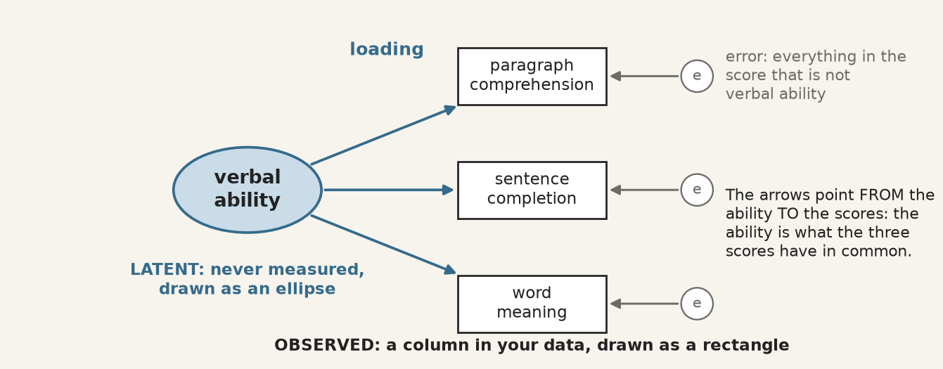
One construct, three indicators. The construct is never measured; it is what the three scores have in common, and the error circles hold everything else in each score.
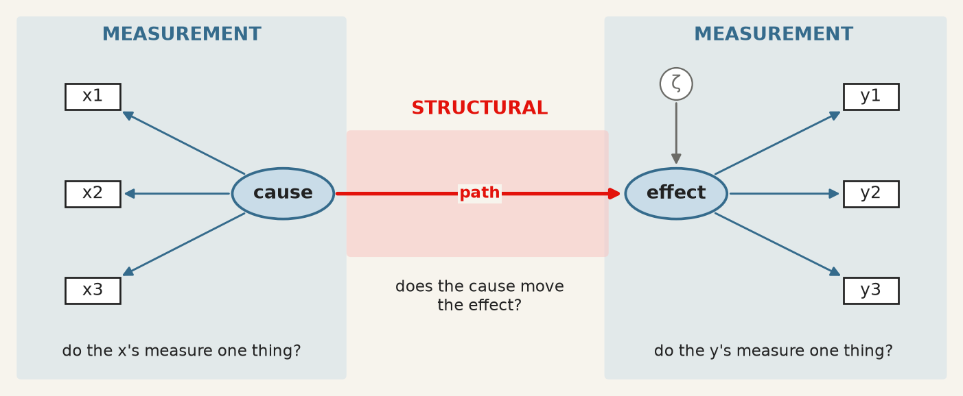
The apparatus divides into two parts, and keeping them apart is the first thing to learn.
Measurement model — the part that links unobserved constructs to observed indicators. It answers: does this battery of questions measure one thing, and how well does each item measure it? Its coefficients are loadings.
Structural model — the part that links constructs to each other. It answers: does this construct predict that one? Its coefficients are path coefficients, and they are regression coefficients between quantities that were never observed.
The two halves of a structural equation model. Blue, the measurement models: does each set of indicators measure one thing? Red, the structural model: does one construct move the other? ζ stands for what the path leaves unexplained.
A model can have both, and much of what makes SEM valuable is estimating them jointly: the structural relationships are corrected for the unreliability of the measurement, which a two-step approach of “build a scale, then regress it” does not do.
9.2 Wright’s diagrams, and what a path meant
From the archive · Wright, 1918–1934
Sewall Wright was a geneticist working on the inheritance of coat colour in guinea pigs, and he needed to express something regression could not: a system in which variables cause each other in a specified pattern, some directly and some through intermediaries. He drew it — variables as boxes, causal claims as arrows — and worked out the algebra that lets the correlations be decomposed along the paths (Wright 1934).
Two features of that invention survive intact into every SEM package in use today. The diagram is the model: each arrow is a parameter to be estimated, and an arrow you do not draw is a claim that the effect is zero. And the implied correlation between any two variables is the sum of the contributions along every path connecting them, which is what makes the model testable — it predicts a whole covariance matrix, not a single coefficient.
Wright was explicit that the method could not discover the diagram. It required the causal structure to be supplied from outside, on subject-matter grounds, and it then estimated the strengths and checked the implications. Ninety years of software has not changed that, and the section on equivalent models below is what happens when it is forgotten.
9.3 The language: five symbols and three operators
Wright’s convention is still universal. Observed variables are rectangles, unobserved ones ellipses, a one-headed arrow is a directed effect, a two-headed arrow an unanalysed covariance, and a small circle the error left over.
The five symbols of a path diagram. Every SEM figure in every paper is made of these.
Each drawing has an exact translation into text. The notation, standard since lavaan made it so (Rosseel 2012) and used by semopy in Python, is close to readable English:
You draw
You write
operator means
ellipse → rectangles
visual =~ x1 + x2 + x3
=~is measured by
ellipse → ellipse
dem65 ~ dem60
~is regressed on
two-headed arrow
y1 ~~ y5
~~covaries with
error circles
nothing
added by the software, one per indicator
So visual =~ x1 + x2 + x3 asserts that a construct called visual exists, that these three observed scores are reflections of it, and — by what is absent — that nothing else in the model measures it. The corresponding equation for indicator \(j\) of construct \(\xi\) is
with \(\lambda_j\) the loading and \(\delta_j\) everything specific to that indicator: its own content, and its measurement error. This is chapter 7’s factor model written one indicator at a time, and the interpretive move is the same — the construct is what the indicators have in common, and nothing else.
Identification. A latent variable has no units, so a scale must be imposed before anything can be estimated. Two conventions exist: fix one loading to 1, which gives the construct the units of that indicator, or fix the construct’s variance to 1, which makes it standardised. Software picks the first by default, which is why one loading in every output has no standard error — it was not estimated. Reading it as “the strongest indicator” is a common and complete misunderstanding.
9.4 What is actually being fitted
The model does not fit the data. It fits the covariance matrix of the data.
Every parameter set \(\theta\) implies a covariance matrix \(\Sigma(\theta)\) among the observed variables, and estimation chooses \(\theta\) to make that as close as possible to the observed \(S\). The simplest case shows why a diagram is a prediction. Standardise everything; two indicators of the same construct share nothing but the construct, so the model says their correlation must be
Every arrow you draw, and every one you leave out, implies a number of this kind for every pair of indicators. The discrepancy between those numbers and the observed ones is what all the fit statistics measure, and the \(\chi^2\) test is a formal test of
\[
H_0: \thickspace \Sigma = \Sigma(\theta) ,
\]
that is, of exact fit. Its degrees of freedom are the number of distinct elements in the covariance matrix minus the number of free parameters: nine indicators have \(9 \times 10 / 2 = 45\) variances and covariances, the three-factor model below estimates 21 parameters, and the 24 left over are what make it testable. A model that says more about the covariances than it has parameters to absorb can be wrong, and therefore can be checked.
9.5 Building a measurement model, step by step
The data are the classic of the field: Holzinger and Swineford gave nine ability tests to 301 seventh- and eighth-graders in two Chicago schools in 1939. They ship with semopy, so every cell below runs as written, with nothing to download.
Column
Test
Meant to measure
x1 · x2 · x3
visual perception · cubes · lozenges
visual ability
x4 · x5 · x6
paragraph comprehension · sentence completion · word meaning
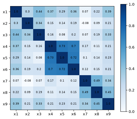
Step 1 and 2 · Load the data, and look before you model. The correlation matrix is what the model will try to reproduce, so it is the first thing to see.
Run it: the correlations the model has to reproduce
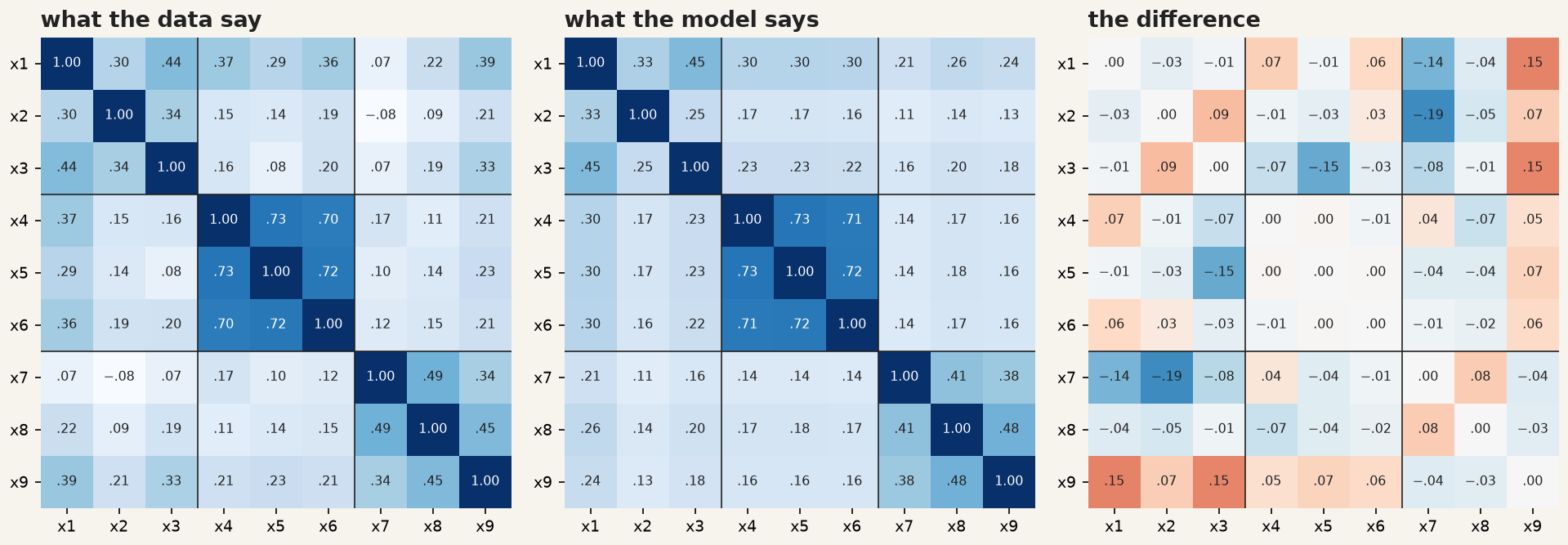
Figure 9.1: The correlations between the nine tests. Three blocks on the diagonal: the groups are visible before any model is fitted.
Three dark squares sit on the diagonal. The textual tests correlate at about 0.7 with each other and 0.1–0.4 with everything else; the visual and speed tests form weaker blocks. If you cannot see your constructs in this picture, no fit index will find them for you.
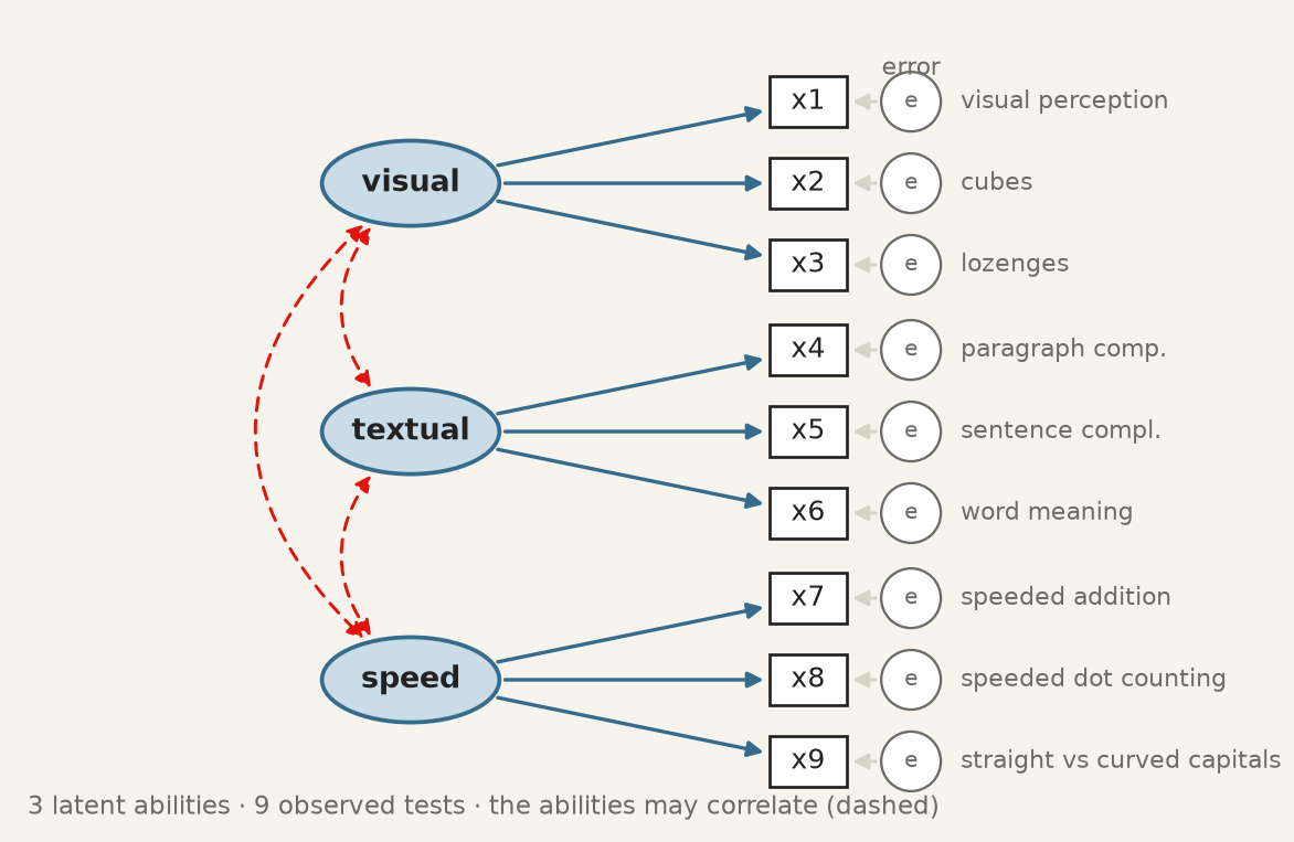
Step 3 · Draw the model on paper. Each test measures one ability, and the three abilities may correlate. Every missing arrow is a claim: no arrow from visual to x9 says the capitals test has nothing to do with visual ability.
The three-factor model, before any number is estimated.
Step 4 and 5 · Write it as text, and fit it. One line per ellipse. semopy adds the rest: one loading per construct fixed to 1, an error term for each indicator, and covariances among the constructs.
Run it: fit the three-factor model and read the loadings
semopy writes a loading as x2 ~ visual — “x2 depends on visual”, which is what =~ means read from the other side. Estimate is in the indicator’s own units, and the rows equal to 1 with no \(p\)-value are the ones fixed in step 4. Est. Std is the column to read: a standardised loading is the correlation between the indicator and its construct, and its square is the share of the indicator the construct explains.
Step 6 · Put the numbers back on the drawing.
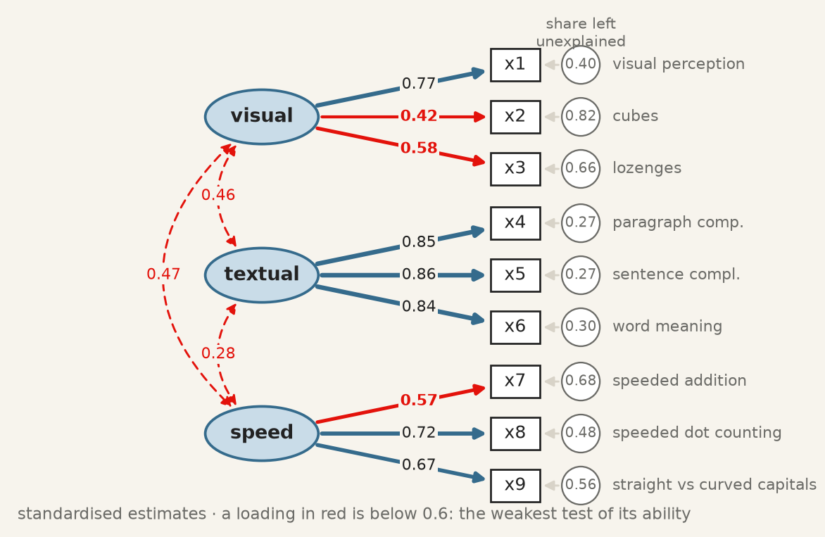
The fitted three-factor model, standardised. Red loadings are below 0.6; the circles hold the share of each test the model leaves unexplained, which is one minus the squared loading.
Textual is measured well, each test sharing about 72% of its variance with the construct. Cubes, x2, is the weak indicator: \(0.42^2 = 0.18\), so 82% of a child’s cubes score is something other than visual ability. Below about 0.4 an item has little to do with the thing it is supposed to measure, and keeping it degrades the construct rather than enriching it.
The rule from the previous section can be checked by hand. x4 and x5 both measure textual, so the model says their correlation is \(0.85 \times 0.86 = 0.73\) — and the correlation in the first figure is 0.73. The three abilities correlate at 0.28 to 0.47: related, but distinct.
9.6 The fit indices, and what each would have to be
The \(\chi^2\) test is the only one with a null hypothesis, and it is almost never used alone, for a reason worth being honest about: with a large sample it rejects models that are approximately right, and with a small one it fails to reject models that are badly wrong. It is a test of exact fit, and no model is exactly right.
The alternatives are approximate fit indices, and three are conventionally reported together.
CFI — comparative fit index (Bentler 1990). How far the model has moved from a baseline in which all observed variables are uncorrelated, toward perfect fit. Scaled to \([0,1]\); above about 0.95 is the modern convention.
TLI — Tucker–Lewis index, the same comparison with a penalty for parameters, so adding a path that does not help can lower it. Not bounded above by 1 in practice. Above about 0.95.
RMSEA — root mean square error of approximation (Browne and Cudeck 1992). The misfit per degree of freedom, so it rewards parsimony directly. Below about 0.06 is good, above 0.10 poor.
Those thresholds come from a simulation study (Hu and Bentler 1999) that has been cited tens of thousands of times and whose authors were careful to say they were not proposing universal cut-offs. They are conventions, and the honest use is to report the numbers and the convention together, and let the reader apply their own judgement.
Run it: every fit index of the three-factor model
fit = semopy.calc_stats(model)print(fit[["chi2", "DoF", "chi2 p-value", "CFI", "TLI", "RMSEA"]].T.round(3))
A model drawn from a well-established theory of mental abilities, and it does not quite fit. That is a normal outcome, and the useful question is where it misses.
9.7 Where the model misses, and what you may do about it
The model implies a correlation for every pair of tests. Subtracting it from the observed one shows where the diagram is wrong.
Observed correlations, the correlations the fitted model implies, and their difference. The textual block is reproduced almost exactly; the largest misses are in the last row, where x9 correlates with the visual tests more than the model allows.
x9 correlates with x1 and x3 by about 0.15 more than the model allows. Is there a reason? The test asks children to tell straight from curved capital letters, quickly: a speed task that also needs visual discrimination. An arrow from visual to x9 can therefore be argued from what the test is, not merely from the numbers. Comparing it with the alternatives is one loop:
Run it: one factor, three factors, and three with x9 on visual
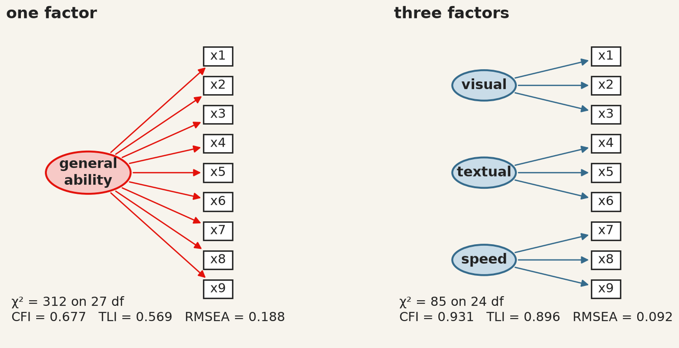
One general ability against three. The single factor is rejected on every index: the tests do not all measure one thing.
One general ability is rejected decisively. Three abilities are far better, and x9 on visual as well brings CFI to 0.967 and RMSEA to 0.065.
What to do about a failing model. Not, in the first instance, to modify it until it passes. Software offers modification indices — the improvement in \(\chi^2\) from freeing each fixed parameter — and following them is how a theoretical model becomes an atheoretical one that fits this sample. The third model above was chosen after looking at the misfit, which makes it exploratory however good its argument. The honest check is data it has not seen. The two schools give a partial one:
Run it: does the x9 change help in each school separately?
for school in ["Pasteur", "Grant-White"]: one_school = data[data["school"] == school]for name in ["three factors", "three + x9 vis"]: m = semopy.Model(models[name]) m.fit(one_school) s = semopy.calc_stats(m)print(f"{school:12} n = {len(one_school)}{name:15} CFI = {s['CFI'].iloc[0]:.3f}"f" RMSEA = {s['RMSEA'].iloc[0]:.3f}")
Pasteur      n = 156  three factors   CFI = 0.903  RMSEA = 0.104
Pasteur      n = 156  three + x9 vis  CFI = 0.927  RMSEA = 0.092
Grant-White  n = 145  three factors   CFI = 0.941  RMSEA = 0.089
Grant-White  n = 145  three + x9 vis  CFI = 0.989  RMSEA = 0.040
In Grant-White the modified model fits well (CFI 0.989, RMSEA 0.040). In Pasteur it helps but still falls short (CFI 0.927, RMSEA 0.092). The change is real in one school and only partial in the other — a finding about the tests, and the kind of result that a single pooled fit would have hidden.
9.8 Adding the structural part
A measurement model says what the constructs are. A structural model says what they do to each other. Bollen’s political-democracy data (Bollen 1989), also bundled with semopy, are the standard example: 75 developing countries, with industrialisation in 1960 measured by three indicators and democracy measured by the same four expert ratings in 1960 and again in 1965.
Construct
Indicators
ind60 · industrialisation, 1960
x1 GNP per capita · x2 energy per capita · x3 share of labour in industry
dem60 · democracy, 1960
y1 press freedom · y2 freedom of opposition · y3 fair elections · y4 effective legislature
dem65 · democracy, 1965
y5–y8: the same four questions, five years later
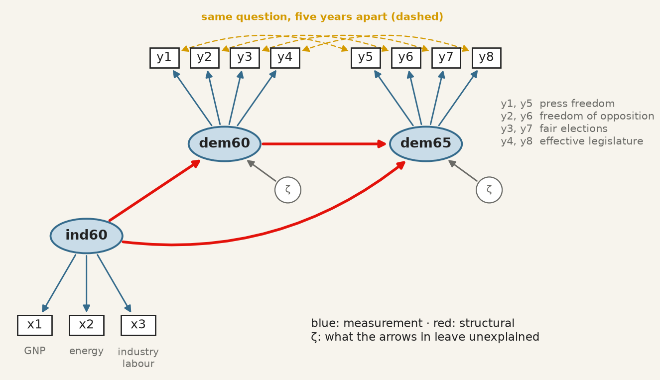
The theory supplies three structural claims: industrialisation raises democracy, democracy persists, and industrialisation may also act on 1965 directly. The design supplies one more. y1 and y5 are the same question, rated by the same experts, so whatever makes a rater generous on press freedom in 1960 plausibly does so again in 1965: their errors may covary. That is decided before fitting, from how the data were collected.
The democracy model before fitting. Blue arrows are measurement, red arrows structural, gold dashed arrows the same question asked twice.
All three operators now appear in one description:
Run it: measurement, structure and covariances in one model
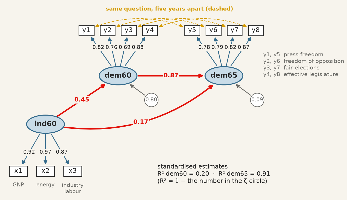
The fitted democracy model, standardised. The numbers in the ζ circles are the unexplained shares, so R² is one minus each.
A country one standard deviation more industrialised in 1960 was 0.45 standard deviations more democratic that year. Democracy is very persistent (0.87), and industrialisation adds a smaller direct push to 1965 on top of that persistence (0.17, \(p = 0.015\)). Industrialisation explains 20% of the variance of democracy in 1960; with 1960 democracy it explains 91% of 1965. All eleven loadings exceed 0.69.
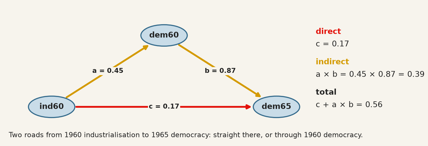
Direct and indirect effects. Industrialisation reaches 1965 by two roads: straight there, and through 1960 democracy. Along a road, standardised paths multiply.
Two routes from ind60 to dem65: the direct path c, and the indirect route a × b through dem60.
Run it: direct, indirect and total effect
a = est.loc[(est["lval"] =="dem60") & (est["rval"] =="ind60"), "Est. Std"].iloc[0]b = est.loc[(est["lval"] =="dem65") & (est["rval"] =="dem60"), "Est. Std"].iloc[0]c = est.loc[(est["lval"] =="dem65") & (est["rval"] =="ind60"), "Est. Std"].iloc[0]print(f"direct c = {c:.2f}")print(f"indirect a * b = {a:.2f} * {b:.2f} = {a * b:.2f}")print(f"total c + a * b = {c + a * b:.2f}")
direct    c         = 0.17
indirect  a * b     = 0.45 * 0.87 = 0.39
total     c + a * b = 0.56
Two-thirds of the total effect (0.39 of 0.56) runs through 1960 democracy: a mediation, in which dem60 carries most of what industrialisation does for dem65. The arithmetic is exact within the model; whether it is a causal decomposition depends entirely on whether the arrows are, which is the subject of the next two sections.
Every extra arrow needs a reason. The four same-question covariances changed the fit, and it is worth seeing by how much:
Run it: the model with and without the same-question covariances
without  chi2 =  72.5  df = 41  p = 0.002  CFI = 0.953  RMSEA = 0.102
with     chi2 =  50.8  df = 37  p = 0.064  CFI = 0.980  RMSEA = 0.071
With them, \(\chi^2\) no longer rejects (\(p = 0.064\)), CFI reaches 0.980 and RMSEA 0.071, and the structural paths barely move. They are legitimate here because the design predicts them. The same four lines added because they raise the CFI would be fitting noise — and correlated residuals added until a model passes are the most common way an SEM paper overstates its evidence.
9.9 What the estimator assumes
Nothing above said how \(\theta\) is chosen. The default, in semopy as in lavaan, is maximum likelihood, and the likelihood it maximises is the multivariate normal one. That assumption is not decoration: the \(\chi^2\) statistic and every standard error in the output are derived from it.
When the data are not multivariate normal — and survey items with floor or ceiling effects rarely are — the failure runs in one direction, which is what makes it dangerous. The \(\chi^2\) statistic is inflated, so a model that fits is rejected. The standard errors are too small, so paths look more significant than they are. Non-normality does not make you cautious. It makes you confident.
The first check is one test per indicator, with functions you already have:
Run it: Shapiro–Wilk, skewness and kurtosis for each test
from scipy import statsfor t in tests: W, p = stats.shapiro(data[t])print(f"{t} W = {W:.3f} p = {p:.4f} skew = {data[t].skew():5.2f}"f" excess kurtosis = {data[t].kurt():5.2f}")
x1  W = 0.993  p = 0.1582  skew = -0.26  excess kurtosis =  0.36
x2  W = 0.970  p = 0.0000  skew =  0.47  excess kurtosis =  0.38
x3  W = 0.952  p = 0.0000  skew =  0.39  excess kurtosis = -0.89
x4  W = 0.983  p = 0.0011  skew =  0.27  excess kurtosis =  0.12
x5  W = 0.977  p = 0.0001  skew = -0.35  excess kurtosis = -0.53
x6  W = 0.954  p = 0.0000  skew =  0.87  excess kurtosis =  0.88
x7  W = 0.991  p = 0.0560  skew =  0.25  excess kurtosis = -0.27
x8  W = 0.981  p = 0.0004  skew =  0.53  excess kurtosis =  1.24
x9  W = 0.994  p = 0.3070  skew =  0.21  excess kurtosis =  0.34
Six of the nine tests reject univariate normality at the 1% level, though none is far from it: the skewness stays below 0.9 and the excess kurtosis below 1.3, small enough that maximum likelihood is a defensible default here. Passing one indicator at a time is not the assumption actually being made, which is joint. Mardia’s measures of multivariate skewness and kurtosis,
test it directly; under normality \(b_2\) has mean \(k(k+2)\), and every indicator can pass Shapiro–Wilk while the joint distribution fails both.
The answer to non-normality is not to abandon the model but to change the estimator. Robust maximum likelihood — MLR, resting on the Satorra–Bentler scaled \(\chi^2\) — keeps the ML point estimates and rescales the test statistic and the standard errors by the non-normality actually observed. For ordinal indicators, WLSMV treats a five-point item as a coarsened continuous variable rather than pretending its categories are numbers. Either way, report the estimator alongside the fit.
9.10 Good fit is not evidence that the model is correct
This is the chapter’s most important section and the objective most often recited without being understood.
A model that fits well has demonstrated one thing: the covariances it implies are close to the covariances observed. It has not demonstrated that its causal structure is right, because other models — with different, even opposite, causal claims — can imply exactly the same covariance matrix. They are called equivalent models, they exist for almost every model anyone fits, and no amount of data distinguishes them.
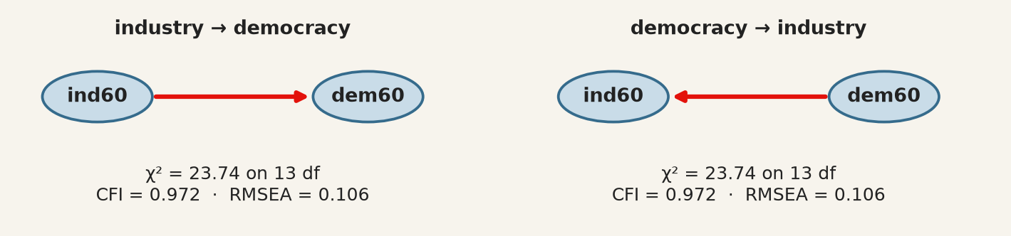
Run it: industry causes democracy, and democracy causes industry
Identical \(\chi^2\), identical degrees of freedom, identical CFI and RMSEA — for two models asserting opposite causal directions. No fit index can prefer one, because fit indices measure distance from the observed covariances and both reproduce them equally.
This is the same structural fact as chapter 7’s rotation indeterminacy, in a more dangerous costume: there, the alternatives were obviously arbitrary and everyone knew a rotation had been chosen; here, the alternative is a different theory of how the world works, and the output looks like a result.
The consequence for practice is exact. The direction of the arrows is an assumption you supply, and the fit statistics cannot audit it. What can audit it is subject knowledge, temporal order — a cause cannot follow its effect, which is why the 1960-to-1965 arrow is more defensible than the 1960-to-1960 one — and design, which is what chapters 10 and 11 are about.
9.11 What SEM does not fix
It does not make cross-sectional data longitudinal. Estimating a path from \(A\) to \(B\) measured at the same moment identifies a direction only because you declared one.
It does not remove confounding. An omitted common cause of two constructs biases the path between them exactly as it biases a regression coefficient. The latent variables absorb measurement error, not confounders.
It is demanding of sample size. With a small \(n\) the \(\chi^2\) test has little power to reject a wrong model, and the fit indices are themselves unstable — so “good fit” in a small sample is the weakest possible evidence. Bollen’s 75 countries are a small sample, and the good fit of the democracy model should be read with that in mind.
Comparisons across groups require an extra assumption. Comparing a construct between, say, countries presumes it is measured the same way in each. That is measurement invariance, it is testable by fitting the model with loadings constrained equal across groups, and comparing means without testing it can manufacture a difference out of a translation (Cheung and Rensvold 2002). The two schools above, where one modification helped in one and not the other, are a small instance of the same problem.
9.12 The recipe
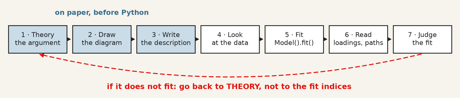
Seven steps from theory to judging the fit. When the model does not fit, the arrow goes back to the theory, not to the fit indices.
Step
What you do
In Python
1–3
argue which indicators measure which construct, draw it, write one line per ellipse
a string with =~, ~, ~~
4
look at the correlations: can you see your groups?
data[cols].corr(), plt.imshow
5
fit
semopy.Model(description), .fit(data)
6
read loadings and paths, standardised
.inspect(std_est=True)
7
judge the fit, all four indices
semopy.calc_stats(model)
9.13 A short review of the literature
The method has two ancestors that met in the 1970s. Wright (1934) developed path analysis in genetics, with the diagram as the model and the decomposition of correlations along paths; Spearman (1904) and the factor-analytic tradition supplied latent variables measured by indicators. Jöreskog (1971) combined them into the general covariance-structure model that all current software implements, Bollen (1989) wrote the textbook that taught a generation to use it — the political-democracy model above is its running example — and Rosseel (2012) gave the modern open-source implementation whose syntax semopy follows in Python.
Assessment of fit is where the applied literature has moved most. Bentler (1990) introduced the comparative fit index and Browne and Cudeck (1992) the RMSEA, both as responses to the chi-square test’s sensitivity to sample size. Hu and Bentler (1999) proposed the cut-offs now universally quoted — CFI and TLI above 0.95, RMSEA below 0.06 — while cautioning against exactly the mechanical application that followed.
MacCallum and Austin (2000) reviewed a decade of applied practice and found the recurring faults to be the ones this chapter warns about: models modified until they fit and then reported as though specified in advance, equivalent models never considered, and causal language attached to cross-sectional designs. Cheung and Rensvold (2002) supplies the invariance testing that any cross-group comparison requires and most omit.
9.14 What to report
The model, as a diagram or as its description. Every arrow is a claim; a reader cannot evaluate claims they cannot see.
How the latent scale was set — a fixed loading or a fixed variance — so nobody misreads the parameter without a standard error.
Standardised loadings for every indicator, not only the significant ones, and what you did about weak items. Dropping an indicator after seeing its loading is a data-dependent decision; say so.
The chi-square with its degrees of freedom and p-value, alongside CFI, TLI and RMSEA, and the convention you judged them against. Reporting only the indices that pass is the single most common failure.
Whether the model was modified after fitting, and on what grounds. A model reached through modification indices or residuals is exploratory whatever its fit, until it holds on data it has not seen.
At least one equivalent model, named. If you cannot think of one, that is a reason to look harder rather than evidence there is none.
What the arrows do not license. Direction was assumed, not discovered. With cross-sectional data the model estimates the strength of a relationship under a causal structure you supplied, and a good fit is consistent with that structure being wrong.
Browne, Michael W., and Robert Cudeck. 1992. “AlternativeWays of AssessingModelFit.”SociologicalMethods & Research 21 (2): 230–58. https://doi.org/10.1177/0049124192021002005.
Cheung, Gordon W., and Roger B. Rensvold. 2002. “EvaluatingGoodness-of-FitIndexes for TestingMeasurementInvariance.”StructuralEquationModeling: A MultidisciplinaryJournal 9 (2): 233–55. https://doi.org/10.1207/S15328007SEM0902_5.
Hu, Li‐tze, and Peter M. Bentler. 1999. “Cutoff Criteria for Fit Indexes in Covariance Structure Analysis: Conventional Criteria Versus New Alternatives.”StructuralEquationModeling: A MultidisciplinaryJournal 6 (1): 1–55. https://doi.org/10.1080/10705519909540118.
Jöreskog, K. G. 1971. “StatisticalAnalysis of Sets of CongenericTests.”Psychometrika 36 (2): 109–33. https://doi.org/10.1007/BF02291393.
MacCallum, Robert C., and James T. Austin. 2000. “Applications of StructuralEquationModeling in PsychologicalResearch.”AnnualReview of Psychology 51 (1): 201–26. https://doi.org/10.1146/annurev.psych.51.1.201.
Rosseel, Yves. 2012. “<B>lavaan</b> : An <i>r</i> Package for StructuralEquationModeling.”Journal of StatisticalSoftware 48 (2). https://doi.org/10.18637/jss.v048.i02.
Spearman, C. 1904. “"GeneralIntelligence," ObjectivelyDetermined and Measured.”TheAmericanJournal of Psychology 15 (2): 201. https://doi.org/10.2307/1412107.