Suppose you have more candidate predictors than you can defend and fewer observations than you would like. The obvious procedure is to let the data choose: start from nothing, add whichever variable improves the fit most, stop when nothing improves it further. That is forward stepwise selection, and variants of it — backward elimination, bidirectional stepwise — were the standard answer for decades and remain the default in a great deal of applied software.
It is worth watching it fail, carefully, because everything in this chapter is a response to the way it fails.
The setting is the wide slice of the course fixtures: thirty-seven complete country-years and twenty-nine candidate predictors. The fixture was built deliberately so that selection has something to get wrong. Fifteen of the columns are named aux_00 to aux_14; ten of them are pure noise, drawn from a standard normal and unrelated to anything, while every third one carries a weak signal — a quarter of a standard deviation of a real latent factor. We know which is which, because the generator wrote them. That is a luxury no real dataset provides and the whole reason for working with fixtures here.
Run it: forward stepwise, and then the same thing on resamples
import sys, warningssys.path.insert(0, "../slides"); sys.path.insert(0, "..")warnings.filterwarnings("ignore")from plotstyle import setup, CLplt = setup()import numpy as np, pandas as pd, statsmodels.api as sm, qmibfrom collections import Counterwide = qmib.load("angle_c_country").dropna()num = wide.select_dtypes("number").drop(columns=["time"], errors="ignore")y = num["ai_use_any"]X = num.drop(columns=["ai_use_any"])# Ground truth, from scripts/build_spine/make_fixtures.py.signal_aux = {f"aux_{k:02d}"for k inrange(15) if k %3==0}noise_aux = {f"aux_{k:02d}"for k inrange(15)} - signal_auxprint(f"n = {len(num)} candidate predictors p = {X.shape[1]}")print(f" of which pure noise: {len(noise_aux)} weak signal: {len(signal_aux)}")def forward_aic(X, y):"""Add the variable that lowers AIC most, until none does.""" chosen, remaining = [], list(X.columns) best = sm.OLS(y, np.ones((len(y), 1))).fit().aicwhile remaining: scored =sorted((sm.OLS(y, sm.add_constant(X[chosen + [c]])).fit().aic, c)for c in remaining)ifnot scored or scored[0][0] >= best -1e-9:break best, pick = scored[0] chosen.append(pick) remaining.remove(pick)return chosenselected = forward_aic(X, y)false_positives = [c for c in selected if c in noise_aux]print(f"\nstepwise selected {len(selected)} variables")print(f" pure noise among them: {len(false_positives)} — {false_positives}")
n = 37   candidate predictors p = 29
   of which pure noise: 10   weak signal: 5

stepwise selected 14 variables
   pure noise among them: 4 — ['aux_01', 'aux_04', 'aux_10', 'aux_14']
Fourteen variables survive, and four of them are columns of pure noise. That alone might be dismissed as bad luck. The damning result is what happens when the same procedure is run on resamples of the same data.
Run it: how stable is ‘the data chose these variables’?
rng = np.random.default_rng(60033)B, counts =200, Counter()for _ inrange(B): idx = rng.integers(0, len(num), len(num)) counts.update(forward_aic(X.iloc[idx], y.iloc[idx]))print(f"forward stepwise repeated on {B} bootstrap resamples\n")print(f"{'variable':22}{'selected':>10} kind")for name, k in counts.most_common(8): kind ="PURE NOISE"if name in noise_aux else ("weak signal"if name in signal_aux else"real predictor")print(f"{name:22}{k/B:>9.0%}{kind}")print(f"\nvariables selected at least once: {len(counts)} of {X.shape[1]}")
forward stepwise repeated on 200 bootstrap resamples

variable                selected   kind
rd_pct_gdp                  98%   real predictor
ai_use_ge3                  94%   real predictor
has_ai_strategy             90%   real predictor
aux_04                      88%   PURE NOISE
aux_12                      86%   weak signal
barrier_legal               86%   real predictor
aux_10                      86%   PURE NOISE
aux_06                      84%   weak signal

variables selected at least once: 29 of 29
Every one of the twenty-nine candidates is selected in some resample. A column of pure noise is chosen in the high eighties per cent of resamples — as reliably as the genuine predictors. “The data selected these variables” is therefore not a finding. Perturb the data slightly and the data select different ones.
The diagnosis is that stepwise makes a sequence of discrete decisions, each conditional on the last. A variable is either in or out; a marginal difference in fit at step three changes the entire subsequent path. That discreteness is what makes the procedure unstable, and it points at the fix: stop making in-or-out decisions and shrink coefficients continuously instead.
5.2 Why a biased estimator can win
Gauss–Markov said least squares is best among unbiased linear estimators. Chapter 3 treated that as reassurance. Read it again as a restriction: the theorem says nothing about estimators that accept bias, and it leaves open whether one of those might have smaller error overall.
Decompose the expected squared error of an estimate \(\hat\theta\) of a quantity \(\theta\):
Least squares sets the first term to zero exactly. If the second term is large — and with twenty-nine correlated predictors and thirty-seven observations it is enormous — then accepting a little bias to remove a lot of variance is a straightforwardly better trade. That is the entire argument for this chapter, and it is a decision-theoretic argument rather than a statistical convention.
Run it: what unbiasedness costs here
full = sm.OLS(y, sm.add_constant(X)).fit()print(f"OLS on all {X.shape[1]} predictors, n = {len(num)}")print(f" R² {full.rsquared:.4f}")print(f" adjusted R² {full.rsquared_adj:.4f}")print(f" residual d.f. {int(full.df_resid)}")print(f" largest |coef| {np.abs(full.params[1:]).max():,.2f}")print(f" mean std. error {full.bse[1:].mean():,.2f}")print("\nAn R² of 0.99 with seven residual degrees of freedom is not a good fit.")print("It is a model with almost as many parameters as observations.")
OLS on all 29 predictors, n = 37
  R²                 0.9935
  adjusted R²        0.9667
  residual d.f.      7
  largest |coef|     5.78
  mean std. error    0.42

An R² of 0.99 with seven residual degrees of freedom is not a good fit.
It is a model with almost as many parameters as observations.
5.3 Ridge: shrink everything, targeted
Hoerl and Kennard proposed adding a penalty on the squared size of the coefficients (Hoerl and Kennard 1970):
Unlike the lasso below, this has a closed form, and the form is the argument:
\[
\hat\beta^{\text{ridge}} \thickspace=\thickspace (X^\top X + \lambda I)^{-1} X^\top y .
\]
Compare it to \((X^\top X)^{-1}X^\top y\). The only change is \(\lambda I\) added to the diagonal — which is why the method is called ridge, and why it works when least squares cannot: \(X^\top X\) may be singular or nearly so, but \(X^\top X + \lambda I\) is invertible for any \(\lambda > 0\). Ridge is defined even when \(p > n\), where least squares has no unique solution at all.
Run it: ridge from its closed form
from sklearn.preprocessing import StandardScalerfrom sklearn.linear_model import Ridge# Standardisation is not optional — see below.Z = StandardScaler().fit_transform(X)yc = (y - y.mean()).to_numpy()lam =18.67beta_hand = np.linalg.solve(Z.T @ Z + lam * np.eye(Z.shape[1]), Z.T @ yc)beta_sk = Ridge(alpha=lam, fit_intercept=False).fit(Z, yc).coef_print(f"largest |difference| between the formula and sklearn: "f"{np.abs(beta_hand - beta_sk).max():.2e}")# Why the shrinkage is targeted: it acts through the singular values of X.sv = np.linalg.svd(Z, compute_uv=False)print(f"\n{'singular value':>16}{'shrinkage factor':>20}")for s in [sv[0], sv[len(sv)//2], sv[-1]]:print(f"{s:16.3f}{s**2/(s**2+ lam):20.4f}")print("\nDirections in which the data vary a lot are barely touched;")print("directions in which they barely vary are shrunk almost to nothing.")
largest |difference| between the formula and sklearn: 1.44e-15

  singular value    shrinkage factor
          20.890              0.9590
           3.456              0.3901
           0.311              0.0052

Directions in which the data vary a lot are barely touched;
directions in which they barely vary are shrunk almost to nothing.
That last block is the point of ridge and the answer to “why not just multiply every coefficient by 0.9”. In the singular value decomposition of \(X\), the ridge estimate shrinks the component along the \(j\)-th direction by the factor \(d_j^2 / (d_j^2 + \lambda)\). Where the data are informative — large \(d_j\) — the factor is near 1 and almost nothing happens. Where the data barely vary, and the least-squares coefficient is therefore an unstable ratio of noise to a very small number, the factor is near 0 and the coefficient is crushed. The shrinkage goes exactly where the variance problem is.
What ridge does not do is select. Every coefficient becomes smaller; none becomes zero. With twenty-nine candidates you still have twenty-nine.
5.4 Lasso: the corner that produces a zero
Tibshirani’s change is a single character: penalise the sum of absolute values rather than of squares (Tibshirani 1996).
There is no closed form in general, but there is in the case that explains everything. Suppose the predictors are orthonormal, so \(X^\top X = I\) and the least-squares solution is \(\hat\beta^{\text{OLS}}_j = z_j\). The objective then separates into one problem per coefficient, and each has the solution
— the soft-thresholding operator. Read what it does. Every coefficient is pulled toward zero by the same fixed amount \(\lambda/2\), and any coefficient whose least-squares value was smaller than that amount is pulled past zero and held there. The zeros are not a numerical accident. They are what happens when a constant subtraction meets a small number.
Ridge, in the same orthonormal case, gives \(z_j / (1 + \lambda)\) — a proportional shrinkage, which multiplies small coefficients by a factor and therefore never reaches zero.
Run it: derive soft-thresholding, then check it against sklearn
from sklearn.linear_model import Lassodef soft_threshold(z, t):return np.sign(z) * np.maximum(np.abs(z) - t, 0.0)# Build a genuinely orthonormal design so the closed form applies.rng2 = np.random.default_rng(7)n_o, p_o =60, 8Q, _ = np.linalg.qr(rng2.normal(size=(n_o, p_o)))beta_true = np.array([3.0, -2.0, 1.2, 0.4, 0.1, 0.0, 0.0, 0.0])y_o = Q @ beta_true + rng2.normal(0, 0.05, n_o)z = Q.T @ y_o # the OLS solution, since Q'Q = Ilam_o =0.5hand = soft_threshold(z, lam_o /2)sk = Lasso(alpha=lam_o / (2* n_o), fit_intercept=False, max_iter=100000).fit(Q, y_o).coef_print(f"{'OLS':>10}{'soft-threshold':>17}{'sklearn lasso':>16}")for a, b_, c_ inzip(z, hand, sk):print(f"{a:10.4f}{b_:17.4f}{c_:16.4f}")print(f"\nlargest |difference|: {np.abs(hand - sk).max():.2e}")print(f"coefficients set exactly to zero: {(hand ==0).sum()} of {p_o}")
       OLS   soft-threshold   sklearn lasso
    3.0202           2.7702          2.7702
   -2.0371          -1.7871         -1.7871
    1.2302           0.9802          0.9802
    0.5094           0.2594          0.2594
    0.1769           0.0000          0.0000
    0.0586           0.0000          0.0000
   -0.0507          -0.0000         -0.0000
    0.1002           0.0000          0.0000

largest |difference|: 1.11e-15
coefficients set exactly to zero: 4 of 8
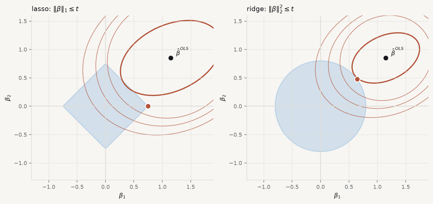
The geometry says the same thing in a picture. Both estimators can be written as minimising the residual sum of squares subject to a budget on the coefficients: \(\lVert\beta\rVert_2^2 \le t\) for ridge, \(\lVert\beta\rVert_1 \le t\) for the lasso. The first constraint region is a disc; the second is a diamond with its corners on the axes. The solution is where the elliptical contours of the residual sum of squares first touch the region — and a diamond is touched at a corner far more often than a disc is touched at a pole, because a corner is where the boundary is not smooth. A corner on the axis means a coefficient of exactly zero.
Figure 5.1: Why the lasso produces zeros and ridge does not. Contours of the residual sum of squares, centred on the least-squares solution, meeting the constraint region. The diamond is touched at its corner, where \(\beta_1 = 0\); the disc is touched at a point with both coordinates nonzero.
5.5 Standardise, always
The penalties are on the size of the coefficients, and a coefficient’s size depends on the units of its predictor. Measure a variable in euros rather than thousands of euros and its coefficient shrinks by a factor of a thousand, so the penalty barely notices it. Nothing about the data changed; the answer did.
Standardising every predictor to mean zero and unit variance before fitting is therefore not hygiene, it is part of the estimator’s definition. The intercept is left unpenalised — there is no reason to shrink the overall level toward zero — which is why it is conventionally handled by centring \(y\) rather than by including a column of ones in the penalty.
5.6 The elastic net, and correlated predictors
The lasso has a specific weakness. Among a group of strongly correlated predictors it tends to pick one, essentially arbitrarily, and zero the rest. If the group is a set of imperfect measurements of the same underlying thing, the choice is close to random, and it will change on a resample — the stepwise instability returning in a new form.
Zou and Hastie’s elastic net penalises both norms at once (Zou and Hastie 2005):
The \(\ell_1\) part still produces zeros; the \(\ell_2\) part produces the grouping effect, under which strongly correlated predictors receive similar coefficients and tend to enter or leave together. \(\alpha = 1\) is the lasso, \(\alpha = 0\) is ridge, and the mixing weight is chosen the same way \(\lambda\) is.
5.7 Choosing \(\lambda\), and what the choice costs
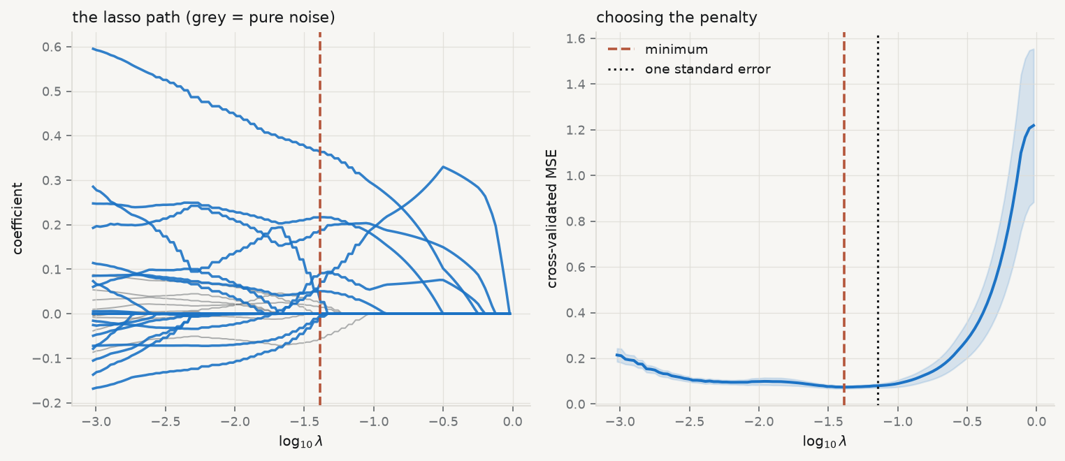
The penalty is not estimated from the fit — a larger \(\lambda\) always fits the training data worse, so anything that rewards fit alone would choose zero. It is chosen by out-of-sample performance, which is what cross-validation estimates (Stone 1974): split the sample into \(K\) folds, fit on \(K-1\), measure error on the held-out fold, rotate, average.
Figure 5.2: Left: the lasso path — every coefficient against the penalty, with the cross-validated choice marked. Coefficients arrive at zero and stay there. Right: the cross-validation curve, with the minimum and the one-standard-error choice.
The dotted line is the one-standard-error rule: rather than the \(\lambda\) with the lowest estimated error, take the largest \(\lambda\) whose error is within one standard error of the minimum. The cross-validation curve is itself an estimate with noise in it, and its minimum is therefore optimistically located. The rule buys a simpler model for an error difference the data cannot resolve.
5.8 Scoring the methods against a known truth
Because the fixture’s generator is known, this is one of the rare occasions when selection methods can be marked rather than admired.
Run it: what each method keeps, against the truth
from sklearn.linear_model import RidgeCV, ElasticNetCVfits = {"ridge": RidgeCV(alphas=np.logspace(-3, 3, 60)),"lasso": LassoCV(cv=5, random_state=0, max_iter=100000),"elastic net": ElasticNetCV(l1_ratio=[.1, .5, .7, .9, .95, .99], cv=5, random_state=0, max_iter=100000),}print(f"{'method':14}{'kept':>6}{'noise kept':>12} penalty")for name, mdl in fits.items(): mdl.fit(Zs, ys) kept = pd.Series(mdl.coef_, index=X.columns) kept = kept[kept.abs() >1e-8] junk = [c for c in kept.index if c in noise_aux] extra =f"λ={mdl.alpha_:.4g}"ifhasattr(mdl, "l1_ratio_"): extra +=f", α={mdl.l1_ratio_}"print(f"{name:14}{len(kept):>6}{len(junk):>12}{extra}")print(f"\nfor reference, stepwise kept {len(selected)} with "f"{len(false_positives)} pure-noise variables")print(f"and there are {len(noise_aux)} pure-noise columns in total")
method          kept  noise kept   penalty
ridge             29          10   λ=18.67
lasso             12           3   λ=0.04122
elastic net       12           3   λ=0.04164, α=0.99

for reference, stepwise kept 14 with 4 pure-noise variables
and there are 10 pure-noise columns in total
Three things in that table are worth stating plainly, including the one that is not flattering.
Ridge keeps everything, as promised — all ten noise columns included, merely with small coefficients. If the deliverable is a shortlist, ridge does not produce one.
The lasso cuts the model from twenty-nine variables to twelve and reduces the pure-noise variables from ten to three. That is a large improvement and it is not a solution. Three noise columns survive cross-validated selection, and a reader told “the lasso selected these twelve” would have no way to know.
The elastic net chose a mixing weight of 0.99 — almost pure lasso — and returned the same model, despite predictor correlations as high as 0.96. That is worth reporting because it contradicts the tidy expectation. Cross-validation optimises predictive error, and the grouping effect buys stability rather than prediction; when the criterion is prediction alone, it will often decline to pay for it.
5.9 What none of this licenses
The chapter’s most important sentence is a prohibition.
A \(p\)-value from a model chosen by the lasso is not a \(p\)-value. Fit the selected variables by ordinary least squares and report the resulting standard errors, and every one of them is wrong — computed as though the specification had been fixed in advance, when in fact it was chosen using the same data.
This is chapter 3’s Freedman problem with a modern face, and it has been treated formally. Valid inference after selection requires either conditioning on the selection event or widening the intervals to cover every model that might have been selected (Berk et al. 2013). Tests designed specifically for the lasso path exist (Lockhart et al. 2014) and are not what a naive refit computes.
The practical responses, in order of how often they are available:
Split the sample. Select on one half, estimate and test on the other. The inference is then honest, at the cost of half the data, and it is the only remedy that needs no theory.
Report stability rather than significance. Refit on many resamples and report the proportion of times each variable is selected (Meinshausen and Bühlmann 2010). That is a statement the data support, and — as the bootstrap at the top of this chapter showed — it is often far less impressive than the single-fit result.
Treat selection as exploratory and say so. A shortlist for further work is a legitimate output. A shortlist presented as a tested finding is not.
5.10 A short review of the literature
Ridge regression begins with Hoerl and Kennard (1970), who proposed biased estimation explicitly as a response to instability under near-collinearity — the title says “biased estimation” without apology. Frank and Friedman (1993) set ridge, subset selection and their relatives in a common framework as members of a family indexed by the power of the penalty, which is where the lasso’s \(\ell_1\) sits between ridge’s \(\ell_2\) and subset selection’s \(\ell_0\).
Tibshirani (1996) introduced the lasso and observed the property that made it dominant: continuous shrinkage and automatic selection in the same estimator. Efron et al. (2004) supplied least angle regression, which computes the entire coefficient path at the cost of a single least-squares fit and turned the lasso from attractive into practical. Zou and Hastie (2005) diagnosed the lasso’s behaviour among correlated predictors and proposed the elastic net, with the grouping effect as the explicit remedy.
Choosing the penalty rests on Stone (1974), whose formulation of cross-validation as a general criterion for model choice long predates its use here.
The inferential warning has the sharpest literature. Berk et al. (2013) established what valid post-selection inference requires and how much wider the intervals must be; Lockhart et al. (2014) developed a test for the lasso path specifically, making clear how different it is from a naive refit. Meinshausen and Bühlmann (2010) offers stability selection as the practical alternative — report how often a variable is chosen across resamples, rather than a significance level that assumes it was never chosen at all.
5.11 What to report
The path, not just the endpoint. A plot of coefficients against \(\lambda\) shows how contingent the chosen model is. If several variables leave within a narrow band of \(\lambda\), say so.
How \(\lambda\) was chosen, with the cross-validation curve, and whether the minimum or the one-standard-error rule was used.
That the predictors were standardised. The estimator is not defined without it.
What survived, and how reliably. Selection frequencies across resamples are worth more than the single selected set.
The prohibition, explicitly. State that the reported coefficients are post-selection and that conventional standard errors and \(p\)-values do not apply to them. If you split the sample, say which half did what.
Why this penalty. Lasso for a shortlist, ridge for prediction under collinearity with no selection wanted, elastic net when correlated groups must move together — and if cross-validation chose an \(\alpha\) near 1 despite correlated predictors, report that rather than the story you expected.
Berk, Richard, Lawrence Brown, Andreas Buja, Kai Zhang, and Linda Zhao. 2013. “Valid Post-Selection Inference.”TheAnnals of Statistics 41 (2): 802–37. https://doi.org/10.1214/12-AOS1077.
Efron, Bradley, Trevor Hastie, Iain Johnstone, and Robert Tibshirani. 2004. “Least Angle Regression.”TheAnnals of Statistics 32 (2): 407–99. https://doi.org/10.1214/009053604000000067.
Hoerl, Arthur E., and Robert W. Kennard. 1970. “RidgeRegression: BiasedEstimation for NonorthogonalProblems.”Technometrics 12 (1): 55–67. https://doi.org/10.1080/00401706.1970.10488634.
Lockhart, Richard, Jonathan Taylor, Ryan J. Tibshirani, and Robert Tibshirani. 2014. “A Significance Test for the Lasso.”TheAnnals of Statistics 42 (2): 413–68. https://doi.org/10.1214/13-AOS1175.
Meinshausen, Nicolai, and Peter Bühlmann. 2010. “StabilitySelection.”Journal of the RoyalStatisticalSocietySeries B: StatisticalMethodology 72 (4): 417–73. https://doi.org/10.1111/j.1467-9868.2010.00740.x.
Stone, M. 1974. “Cross-ValidatoryChoice and Assessment of StatisticalPredictions.”Journal of the RoyalStatisticalSocietySeries B: StatisticalMethodology 36 (2): 111–33. https://doi.org/10.1111/j.2517-6161.1974.tb00994.x.
Tibshirani, Robert. 1996. “RegressionShrinkage and SelectionVia the Lasso.”Journal of the RoyalStatisticalSocietySeries B: StatisticalMethodology 58 (1): 267–88. https://doi.org/10.1111/j.2517-6161.1996.tb02080.x.
Zou, Hui, and Trevor Hastie. 2005. “Regularization and VariableSelectionVia the ElasticNet.”Journal of the RoyalStatisticalSocietySeries B: StatisticalMethodology 67 (2): 301–20. https://doi.org/10.1111/j.1467-9868.2005.00503.x.