Every method so far has assumed a form. Least squares assumes a line, logistic regression assumes a curve, and the penalties in chapter 5 assume the line is worth shrinking toward. Each assumption is a claim that can be wrong, and chapter 3 was about detecting when it is.
Nearest neighbours makes no such claim. To predict for a new observation, find the \(k\) observations in the training data closest to it, and average their outcomes:
where \(N_k(x_0)\) is the set of the \(k\) nearest training points. For a classification problem, take the majority vote instead. There is no fitting stage, no coefficient, no optimisation — the training data is the model.
This looks like getting something for nothing, and the chapter is about what it actually costs. The method is not assumption-free; it has simply moved its assumption. Averaging the neighbours presumes that the function is smooth enough that points close in \(x\) have similar \(y\), and it presumes you know what “close” means. Both presumptions can fail badly, and neither shows up as a diagnostic plot.
No portrait accompanies this chapter. The method is due to Evelyn Fix and Joseph Hodges, in a 1951 technical report for the US Air Force School of Aviation Medicine that went unpublished for nearly forty years (Fix and Hodges 1989), and no freely licensed likeness of either author appears to exist. The convention this book follows is a real portrait or none.
8.2 The floor nobody beats
Before asking how well a classifier does, ask how well anything could.
Bayes classifier — the rule that assigns each \(x\) to the most probable class given \(x\): predict class \(j\) where \(\Pr(Y = j \mid X = x)\) is largest. Its error rate, the Bayes rate, is the lowest achievable by any classifier whatsoever.
The proof is a one-liner: at each \(x\), any rule either picks the most probable class or does not, and picking it minimises the chance of being wrong there. Integrating over \(x\) gives the result.
The Bayes classifier is not a method, because computing it requires \(\Pr(Y \mid X)\) — which is the thing you are trying to estimate. Its value is conceptual and it is considerable. A non-zero Bayes rate means that error is not evidence of a bad model. If the outcome is genuinely uncertain given the predictors, no amount of flexibility, data or cleverness removes the remaining error, and a practitioner who keeps adding complexity to chase it is chasing noise.
The regression analogue is the irreducible error \(\sigma^2\): the variance of \(y\) around \(f(x)\), which no estimator of \(f\) can touch. It appears explicitly in the decomposition below.
8.3 Where prediction error comes from
Take a target \(y = f(x) + \varepsilon\) with \(\mathrm{E}[\varepsilon] = 0\) and \(\mathrm{Var}(\varepsilon) = \sigma^2\). Let \(\hat f\) be an estimate built from a random training sample. The expected squared error at a point \(x_0\), averaged over training samples and over the noise in a new observation, splits into three:
Chapter 5 used the last two terms to argue for a biased estimator. Here all three matter, and the first is the one that makes the others meaningful: because \(\sigma^2 > 0\), the total error has a floor, and the only quantity a modeller controls is how the remaining budget is split between bias and variance.
The words are worth being precise about. Bias is how far the method’s average prediction is from the truth — an error it makes systematically, in every sample. Variance is how much the prediction moves when the training sample changes — an error it makes differently each time. A rigid method has high bias and low variance; a flexible one has the reverse.
For nearest neighbours, \(k\) is the dial. Small \(k\) averages few points, follows the data closely, and changes a lot when the data change: low bias, high variance. Large \(k\) averages many points, smooths across regions where the truth differs, and barely moves between samples: high bias, low variance.
The decomposition is usually presented as algebra and left there. It is measurable, if you are willing to simulate a world whose truth you know.
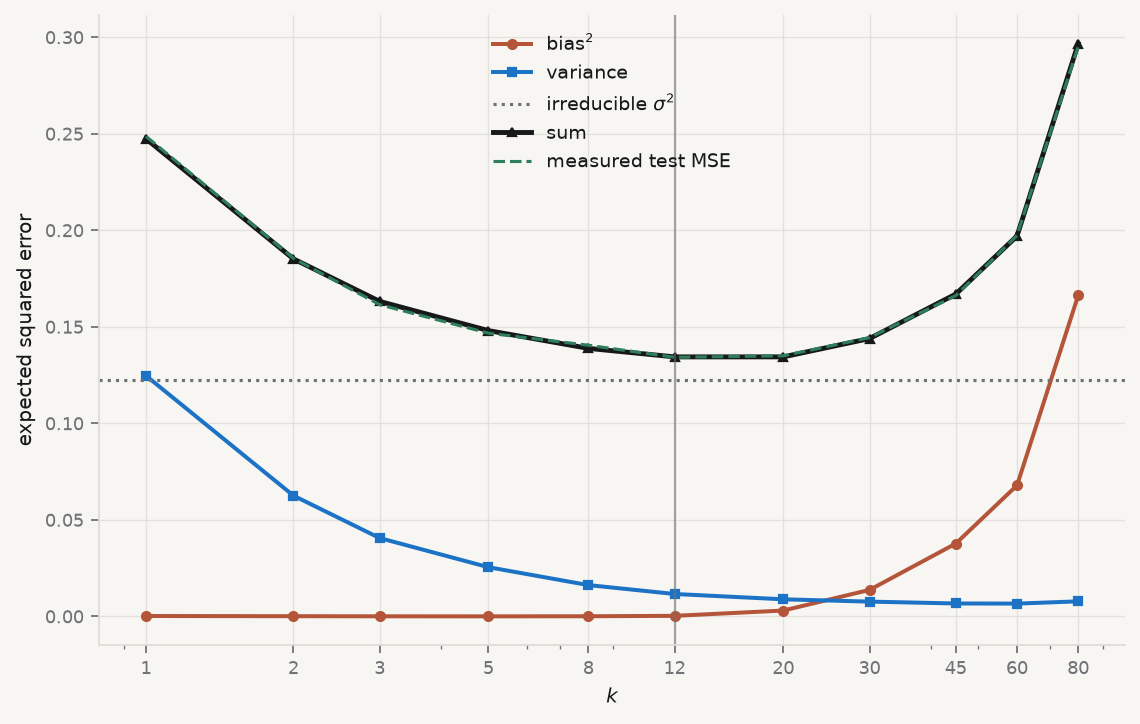
Figure 8.1: The decomposition, measured. Four hundred training samples are drawn from a known function; for each \(k\) the squared bias and the variance of the prediction are computed across samples. Their sum plus the irreducible error tracks the test error to within 0.002 everywhere.
Read the table rather than the shape. Variance falls by a factor of sixteen between \(k = 1\) and \(k = 80\); squared bias rises by a factor of several hundred. The sum is U-shaped with a minimum in between, and the identity holds — the sum of the three estimated components matches the independently measured test error at every \(k\). That is the decomposition being verified, not illustrated.
Note also what happens at the extremes. At \(k = 1\) the method has essentially no bias and all the error is variance plus noise. At \(k = 80\), two thirds of the sample is averaged into every prediction and the bias dominates. Neither extreme is a modelling failure; both are the same dial at different settings.
Effective degrees of freedom — for \(k\)-nearest neighbours, roughly \(n/k\). At \(k = 1\) the method has as many effective parameters as observations, which is why it interpolates the training data exactly; at \(k = n\) it has one, and predicts the global mean everywhere. It is the same quantity chapter 5’s penalty controlled continuously.
8.4 Distance is not given, it is chosen
Nearest neighbours needs a definition of “near”. The default is Euclidean distance,
and that formula adds squared differences measured in different units. A difference of one euro and a difference of one index point are treated as identical quantities. In practice the variable with the largest numerical range determines the neighbours entirely, and every other predictor is decoration.
This is the third time this book has reached the same conclusion — PCA in chapter 7, the penalties in chapter 5, and now here — and the reason is always the same: any method that compares magnitudes across variables must first make them comparable. Standardise before computing a distance. The alternative is a method whose answer depends on whether you recorded revenue in dollars or millions of dollars.
8.5 The curse of dimensionality
The deeper problem is that “near” stops existing as the number of predictors grows, and it does so much faster than intuition suggests.
The last column is what matters: the gap between the nearest and the farthest point, relative to the nearest. In one dimension the farthest point is around a thousand times further away than the nearest. By fifty dimensions it is half again as far; by five hundred, a fifth. All the points are approximately the same distance from the query, so “the ten nearest” is close to a random selection of ten (Beyer et al. 1999).
There is a second, geometric way to see the same thing. To capture a fixed fraction \(r\) of the data in a hypercube of \(p\) dimensions, the neighbourhood must span \(r^{1/p}\) of the range of each variable. Capturing 1% of the data needs 10% of the range in two dimensions, 63% in ten, and 95% in a hundred — a “neighbourhood” covering almost the entire space, which is not local in any useful sense.
The consequence for practice is blunt. Nearest neighbours works well with few predictors and abundant data, and degrades quickly as predictors are added. Adding a variable to a linear model costs one parameter; adding one to a nearest neighbour method costs a dimension of the space in which distance must remain meaningful.
8.6 Choosing \(k\), and why training error lies
The training error of \(1\)-nearest-neighbour is exactly zero: every training point is its own nearest neighbour, so it predicts itself perfectly. That number is not a measure of anything, and any procedure that selects \(k\) by fitting error will select \(k = 1\) every time.
Cross-validation is the answer, as it was in chapter 5. Split, fit on the rest, measure on the held-out part, rotate.
Show the code
from sklearn.model_selection import cross_val_score, KFoldxs = rng.uniform(0, 1, 200).reshape(-1, 1)ys = truth_fn(xs.ravel()) + rng.normal(0, SIGMA, 200)grid = [1, 2, 3, 5, 8, 12, 20, 30, 45, 60, 90, 130]train_err, cv_err = [], []for k in grid: m = KNeighborsRegressor(n_neighbors=k).fit(xs, ys) train_err.append(np.mean((ys - m.predict(xs)) **2)) cv_err.append(-cross_val_score(KNeighborsRegressor(n_neighbors=k), xs, ys, cv=KFold(10, shuffle=True, random_state=0), scoring="neg_mean_squared_error").mean())fig, ax = plt.subplots(figsize=(7.0, 4.3))ax.plot(grid, train_err, marker="o", ms=4, lw=1.8, color=CL.muted, label="training error")ax.plot(grid, cv_err, marker="s", ms=4, lw=2.0, color=CL.accent, label="10-fold CV error")ax.axhline(SIGMA **2, ls=":", lw=1.4, color=CL.warn, label=r"irreducible $\sigma^2$")ax.axvline(grid[int(np.argmin(cv_err))], color=CL.ink, lw=1, ls="--")ax.set_xlabel("$k$"); ax.set_ylabel("mean squared error")ax.set_xscale("log"); ax.set_xticks(grid); ax.set_xticklabels(grid)ax.legend(frameon=False, fontsize=8.5)fig.tight_layout()print(f"training error at k=1: {train_err[0]:.6f} (exactly zero — every point is its own neighbour)")print(f"CV chooses k = {grid[int(np.argmin(cv_err))]}, CV error {min(cv_err):.4f}")print(f"irreducible floor σ² = {SIGMA**2:.4f}")
training error at k=1: 0.000000  (exactly zero — every point is its own neighbour)
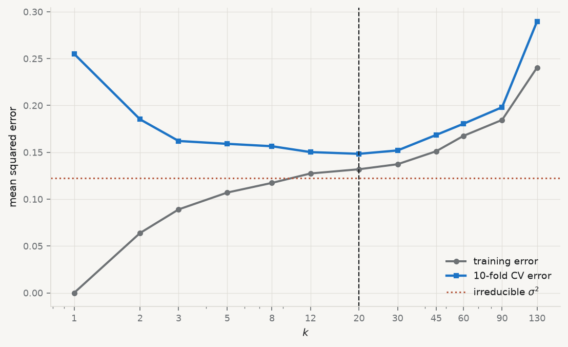
CV chooses k = 20, CV error 0.1484
irreducible floor σ² = 0.1225
Figure 8.2: Training error against cross-validated error for the same data. Training error rises monotonically with \(k\) and is zero at \(k=1\); only the cross-validated curve has a minimum, and it is not at \(k=1\).
Two things are visible. The training curve is monotone and useless for selection. And the cross-validated minimum sits close to, but above, the irreducible floor — which is what a well-tuned method looks like. A cross-validated error below\(\sigma^2\) would indicate a leak between the folds rather than a triumph.
8.7 Did the flexibility earn its keep?
Now the real question, on real data. Nearest neighbours is flexible; flexibility costs variance; and the only justification for paying is that the truth is non-linear in a way a linear model misses. Whether that holds is an empirical question, and it is answered by comparison rather than by assertion.
Run it: kNN against a baseline and against logistic regression
n = 385   base rate = 0.101   majority-class accuracy = 0.8987

model                           accuracy   ROC AUC
kNN, k=5, standardised            0.8909    0.5147
kNN, k=25, standardised           0.8987    0.5609
logistic regression               0.8987    0.6754
The result is unflattering to the method this chapter is about, and it is the most useful output in it.
On accuracy, nothing beats predicting the majority class. All three models score about 0.899, which is exactly what you get by declaring that no country falls behind, ever. Chapter 4 warned about this: with a base rate of 10%, accuracy is a measure of the base rate rather than of the model.
On AUC, the models separate completely. Nearest neighbours at \(k=5\) scores 0.51 — a coin flip, no information whatsoever. At \(k=25\) it recovers to 0.56. Logistic regression, the rigid method with the strong assumption, reaches 0.68.
So the flexibility did not earn its keep. There is signal in these predictors, a linear model finds it, and the flexible method spends its budget on variance and comes back with almost nothing. Had the comparison been made on accuracy alone, all three would have looked identical and the conclusion would have been that nothing works — which is false, and would have been the wrong lesson.
8.8 A worked example: can the market’s past predict today?
The lecture runs one complete prediction exercise, the way it would be done by someone whose job depended on it, and the chapter repeats it here because every step carries a rule. The question is whether the S&P 500’s return two days ago says anything about whether the index rises or falls today. The data are Smarket from An Introduction to Statistical Learning: 1,250 trading days, 2001 to 2005, with the five previous days’ returns (Lag1 to Lag5) and the day’s Direction.
The work is split into two files, because in practice the two jobs happen at different times. The first is the laboratory: it chooses \(K\), judges the model once, and saves it. The second is the trading desk: it loads the saved model and predicts one new date, with no data to download and no training. Both are published with the lecture as session08_1_train.py and session08_2_predict.py.
Two decisions come before any model. One late day, 28 December 2005, is put aside to play “tomorrow”, and the two days after it are dropped, because on the morning of the 28th they are the future. The rest is split by time: the model learns from 2002–2004 and is judged on 2005. A random split would put days of 2005 into the training data, and the model would learn from the future to “predict” the past.
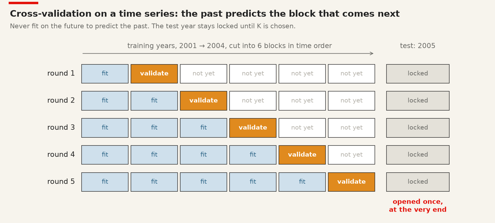
Cross-validation has to respect time as well. The ordinary \(k\)-fold scheme of chapter 5 would fit on 2004 to predict 2002. For a time series each round fits on everything up to a date and validates on the block that follows, which is what scikit-learn’s TimeSeriesSplit does.
Cross-validation on a time series: each round fits on the past and validates on the next block, never the reverse.
Run it: choose K by time-ordered cross-validation
import matplotlib.pyplot as pltimport pandas as pdfrom sklearn.model_selection import TimeSeriesSplit, GridSearchCVfrom sklearn.neighbors import KNeighborsClassifierfrom sklearn.pipeline import make_pipelinefrom sklearn.preprocessing import StandardScalerURL ="https://raw.githubusercontent.com/intro-stat-learning/ISLP/main/ISLP/data/Smarket.csv"smarket = pd.read_csv(URL)smarket = smarket[smarket["Year"] >=2002]predictors = ["Lag2"]new_day, history = smarket.iloc[[-3]], smarket.iloc[:-3] # 28 Dec 2005, and every day beforetrain, test = history[history["Year"] <2005], history[history["Year"] ==2005]X_train, y_train = train[predictors], train["Direction"]X_test, y_test = test[predictors], test["Direction"]# The scaler sits inside the pipeline, so each round standardises on its own fitting rows onlyk_values =list(range(1, 126, 2)) # odd, so a two-class vote cannot tiesearch = GridSearchCV(make_pipeline(StandardScaler(), KNeighborsClassifier()), {"kneighborsclassifier__n_neighbors": k_values}, cv=TimeSeriesSplit(n_splits=5))search.fit(X_train, y_train)best_k = search.best_params_["kneighborsclassifier__n_neighbors"]majority = y_train.value_counts(normalize=True).max()print(f"best K = {best_k}, cross-validated accuracy = {search.best_score_:.3f}")print(f"always predicting the commonest direction = {majority:.3f}")plt.figure(figsize=(7, 3.2))plt.plot(k_values, search.cv_results_["mean_test_score"], "o-", markersize=3, label="KNN, cross-validated accuracy")plt.axhline(majority, color="red", linestyle="--", label="always the commonest direction")plt.axvline(best_k, color="grey", linestyle=":", label=f"chosen K = {best_k}")plt.xlabel("K"); plt.ylabel("accuracy on the hidden blocks")plt.legend(frameon=False, fontsize=8)plt.tight_layout()plt.show()
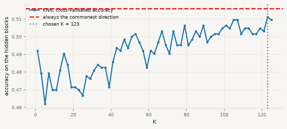
best K = 123, cross-validated accuracy = 0.511
always predicting the commonest direction = 0.516
Figure 8.3: Cross-validated accuracy of KNN on the 2002–2004 training days, for every odd K from 1 to 125, against always predicting the commonest direction. No K clears the line.
The search ran the cross-validation loop for each of 63 values of \(K\) and kept \(K = 123\), with an accuracy of 0.511 on the hidden blocks. “Best” means best of the values tried, not good: it is just below the 0.516 of always predicting the commonest direction. Cross-validation is already saying that Lag2 carries little information about today.
The test year is opened once.\(K\) is now fixed, and only now is 2005 consulted. If \(K\) were changed after seeing this score, 2005 would have become training data and the score would stop being a test.
             predicted Down  predicted Up
actual Down              35            74
actual Up                31           109

KNN accuracy on 2005:                      0.578
always predicting the commonest direction: 0.562
The diagonal holds the right calls, 35 down days and 109 up days, so accuracy is \((35 + 109)/249 = 0.578\), a little better than “always up” at 0.562. Read by row, the model catches 78% of the up days but only 32% of the down days: it says “up” on 183 of 249 days, and much of its accuracy is the market rising more often than not.
Training and predicting are different jobs. Before it is used, the model is refitted on every day it is allowed to know, with the chosen \(K\), and saved to a file. The second script loads that file and predicts the new day from one number, the return two trading days earlier.
Run it: refit on all the history, save, load, and predict one new date
prediction for 28 December 2005: Up
   Pr(Down) = 0.423
   Pr(Up) = 0.577
The probabilities are the votes of the \(K\) nearest past days. The index did rise on 28 December 2005, so the prediction was right — and one date proves nothing either way. The test year is how the model is judged; the second file is how it is used.
How this example was chosen. The example was built to work, and the lecture says so. The natural first attempt — both lags, all five years, the very last day as the new date — scored 50.6% on 2005, below the 56.2% of “always up”, and got its date wrong. So 54 slices of the data were tried (predictors, training years, test year) and one that wins was kept. On 249 test days, accuracy moves by about three points from chance alone (\(\sqrt{0.25/249} \approx 0.032\)); among 54 tries, a winner that beats the baseline by 1.6 points is easy to find with no signal at all. And every look at 2005 made 2005 training data: the test was opened 54 times, not once. This is the garden of forking paths (Gelman and Loken 2014), and it is how most strategies that “beat the market” are found. The steps above are right. The evidence is not.
8.9 What nearest neighbours cannot do
It cannot explain. There are no coefficients, so there is nothing to interpret, no marginal effect, no test of a hypothesis about a mechanism. It is a prediction machine, and chapter 1’s distinction applies with full force.
It cannot extrapolate. A query outside the range of the training data is answered by whichever training points happen to be least far away, which will be the boundary points, no matter how far outside you go. The prediction is confidently wrong and nothing signals it.
It is slow where it matters. Fitting is free and predicting is expensive: the entire training set must be searched for every query. That is the opposite of the profile you usually want in production.
It is exposed to irrelevant variables. Adding a predictor that carries no information does not merely fail to help — it actively corrupts the distances, diluting the informative dimensions. Chapter 5’s penalties can shrink a useless variable to zero; a distance cannot.
8.10 A short review of the literature
The method originates in an unpublished 1951 technical report by Fix and Hodges (1989), whose belated reprinting in 1989 is the citable version. Cover and Hart (1967) proved the result that made it respectable: as the sample grows, the error rate of the 1-nearest-neighbour rule is bounded above by twice the Bayes rate — so the simplest possible classifier, using one point, is asymptotically within a factor of two of the best any method can do. Stone (1977) established the conditions under which nearest-neighbour regression is consistent, completing the theoretical case.
The trade-off itself is stated in its modern form by Geman, Bienenstock, and Doursat (1992), who framed it as a dilemma rather than a choice: any method flexible enough to fit an arbitrary function is flexible enough to fit the noise, and the resolution has to come from outside the data, as a restriction, a penalty, or a tuning parameter chosen by resampling.
Beyer et al. (1999) is the reference for the failure in high dimensions, showing that under broad conditions the distance to the nearest neighbour approaches the distance to the farthest as dimension grows — so the query on which the whole method depends becomes meaningless, not merely imprecise.
8.11 What to report
The baseline first. Majority-class accuracy, or the mean for regression. Every subsequent number is read against it.
A metric the base rate does not dominate. AUC, balanced accuracy or a proper scoring rule. Accuracy on a 10% outcome tells you the outcome is 10%.
How \(k\) was chosen, with the cross-validation curve, and the training curve alongside it if you want to make the point that it is uninformative. With data in time order, say that the folds followed time.
That the test set was opened once, and how many specifications were tried before the one reported. A score found after many looks is not a test score.
That the predictors were standardised, and how many there are. With more than a handful, say what you did about the dimensionality.
The comparison against a rigid model. Flexibility is a purchase, and the report should say what it bought. If a linear model does as well or better, that is the finding.
What the method cannot support. No interpretation, no extrapolation, and no claim about mechanism — only about prediction, within the range of the training data.
Beyer, Kevin, Jonathan Goldstein, Raghu Ramakrishnan, and Uri Shaft. 1999. “WhenIs‘NearestNeighbor’Meaningful?” In LectureNotes in ComputerScience, 217–35. SpringerBerlinHeidelberg. https://doi.org/10.1007/3-540-49257-7_15.
Cover, T., and P. Hart. 1967. “Nearest Neighbor Pattern Classification.”IEEETransactions on InformationTheory 13 (1): 21–27. https://doi.org/10.1109/TIT.1967.1053964.
Fix, Evelyn, and J. L. Hodges. 1989. “DiscriminatoryAnalysis. NonparametricDiscrimination: ConsistencyProperties.”InternationalStatisticalReview / RevueInternationale de Statistique 57 (3): 238. https://doi.org/10.2307/1403797.
Geman, Stuart, Elie Bienenstock, and René Doursat. 1992. “NeuralNetworks and the Bias/VarianceDilemma.”NeuralComputation 4 (1): 1–58. https://doi.org/10.1162/neco.1992.4.1.1.